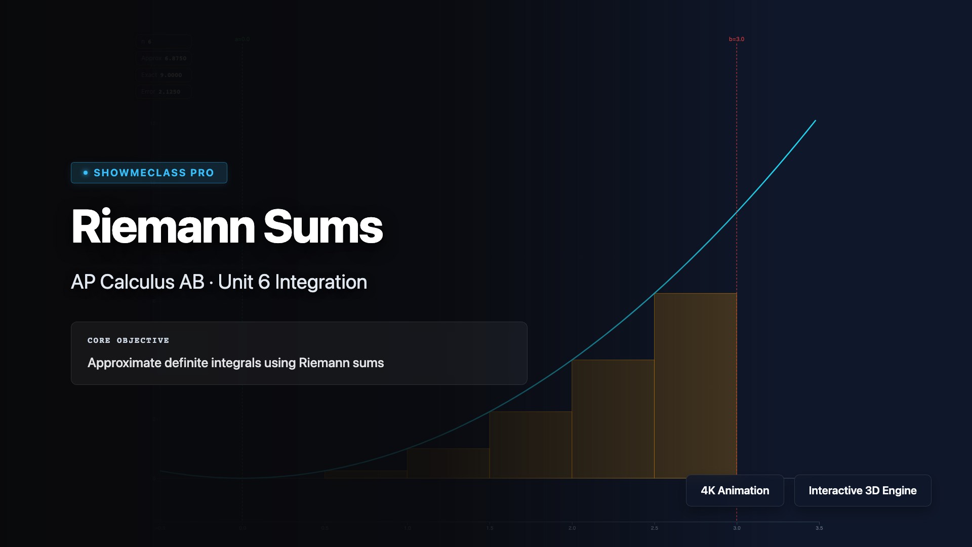
Riemann Sum Explorer
Interactively approximate definite integrals using left, right, and midpoint Riemann sums. Adjust the number of rectangles to watch the approximation converge to the true area under the curve.
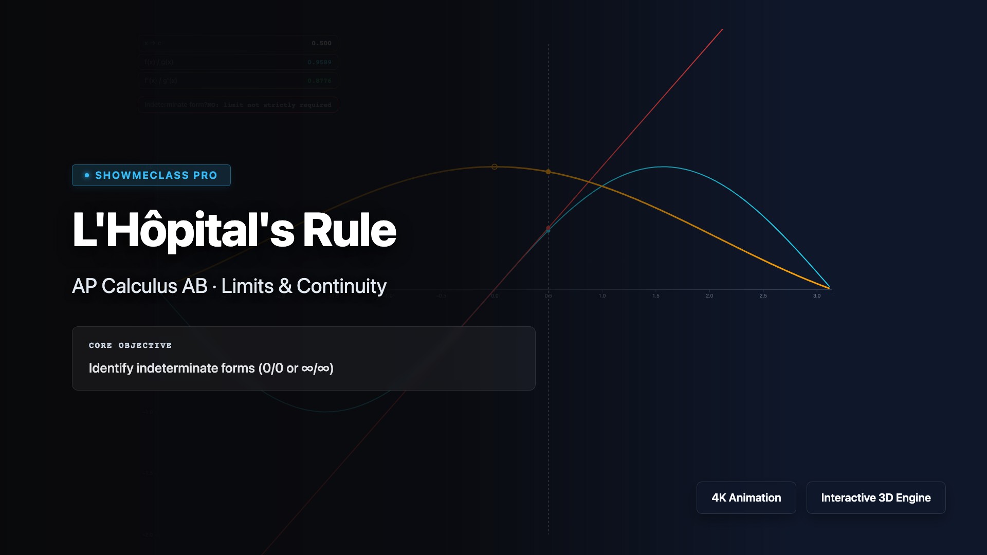
L'Hôpital's Rule
Apply L'Hôpital's Rule to evaluate indeterminate forms like 0/0 and ∞/∞ by taking derivatives of the numerator and denominator. Visualize how lim[x→c] f(x)/g(x) = lim[x→c] f'(x)/g'(x) when the original limit produces an indeterminate form. Practice identifying when to apply the rule, handling repeated applications, and recognizing other indeterminate forms like 0·∞, ∞-∞, 0⁰, 1^∞, and ∞⁰.
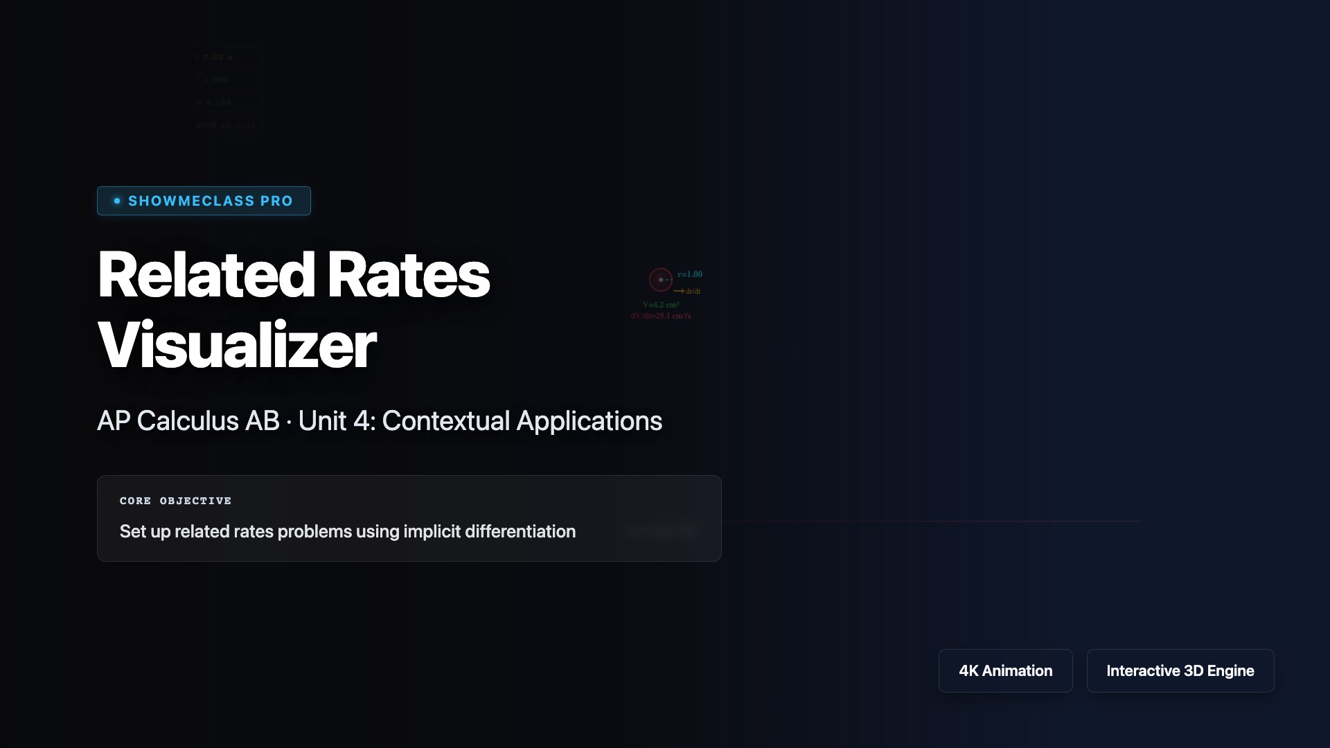
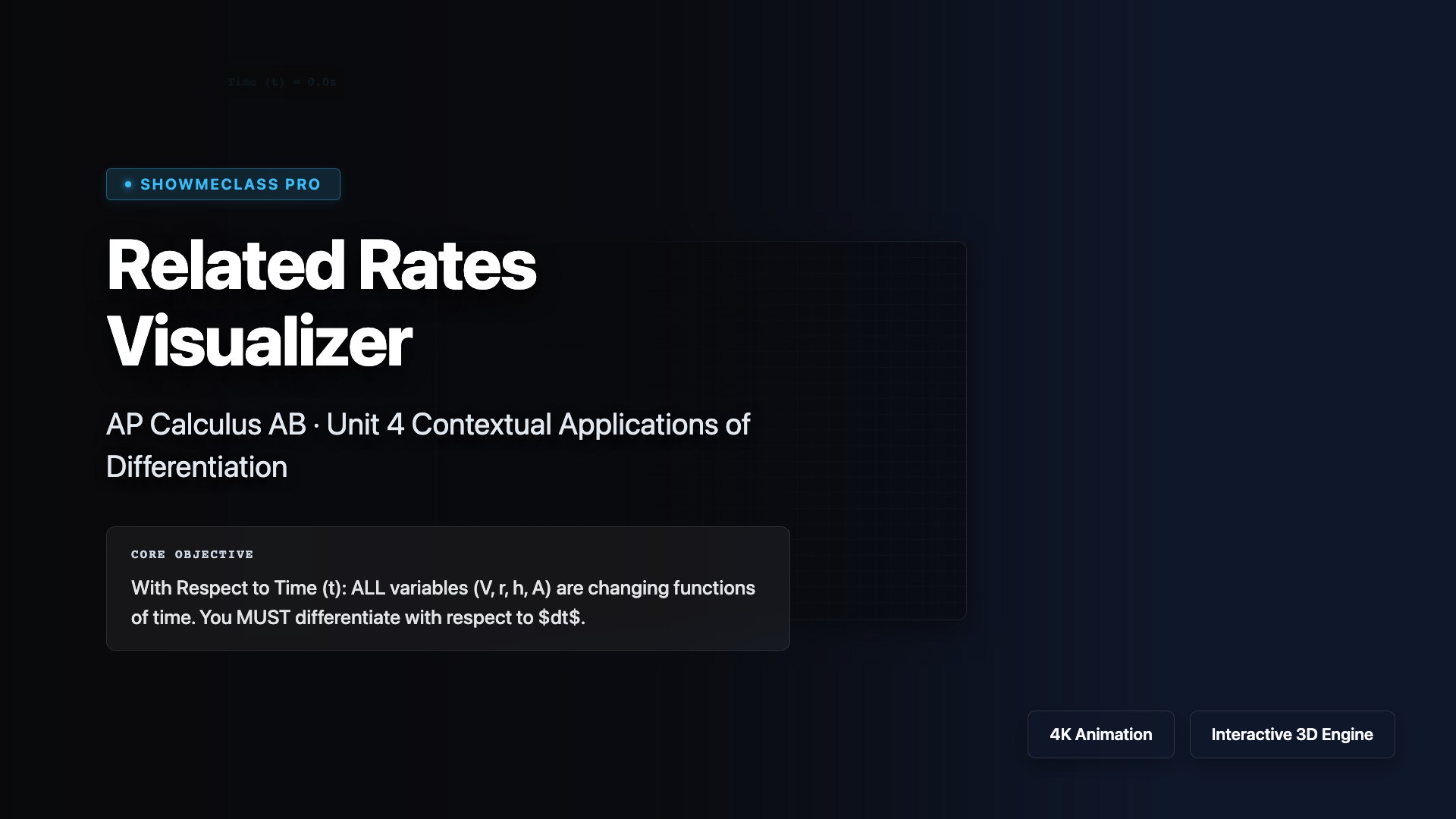
Related Rates Visualizer
Solve related rates problems where multiple quantities change with respect to time and are connected by an equation. Use implicit differentiation with respect to time to find how one rate of change relates to another. Visualize classic scenarios like ladder sliding down walls, water filling conical tanks, expanding circles, and moving shadows, applying the chain rule to connect dy/dt, dx/dt, and geometric relationships.
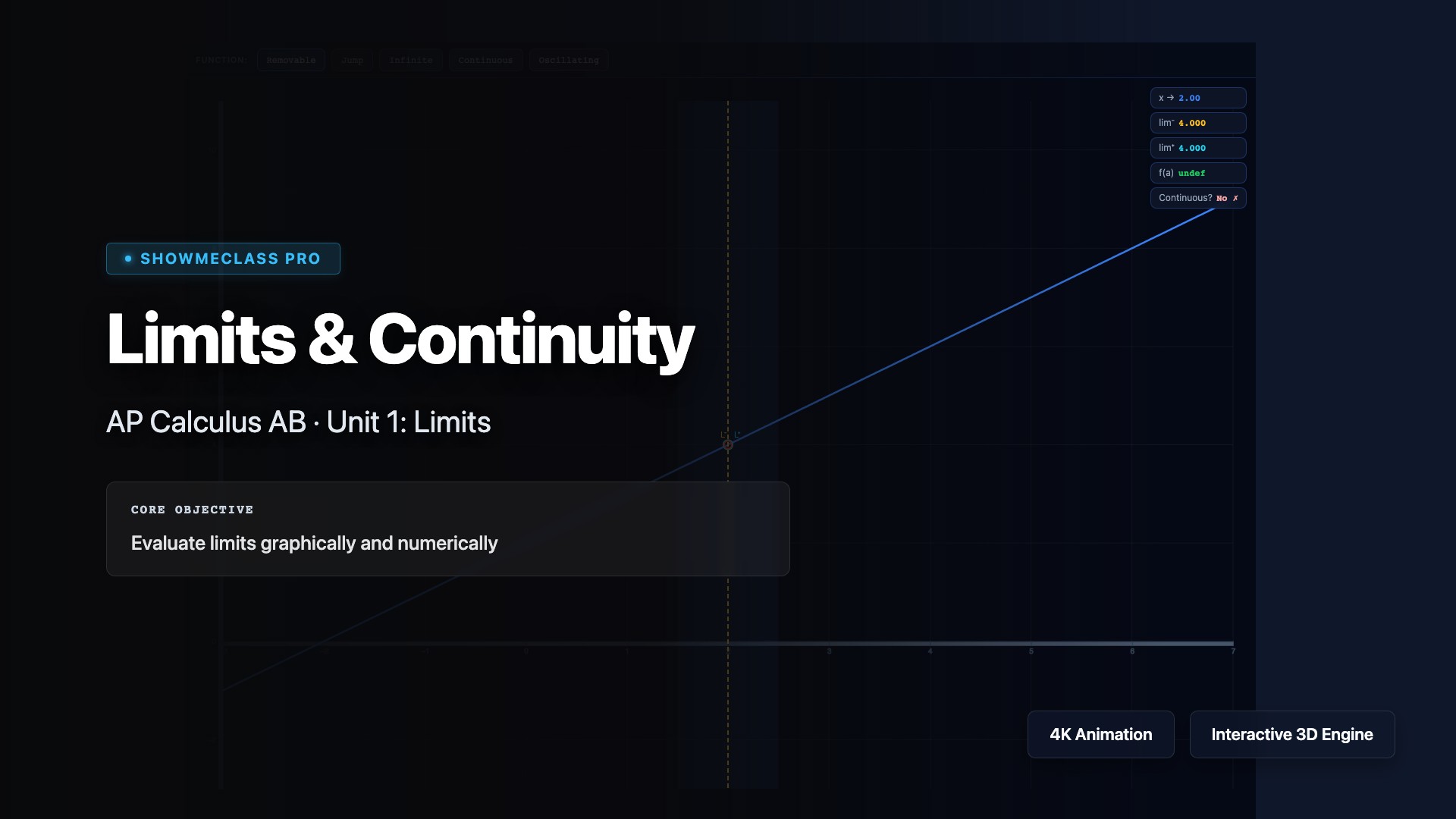
Limits & Continuity
Explore the foundational concepts of limits and continuity that underpin all of calculus. Visualize one-sided limits, two-sided limits, and limits at infinity. Understand the three conditions for continuity at a point: f(c) is defined, lim[x→c] f(x) exists, and lim[x→c] f(x) = f(c). Practice identifying discontinuities (removable, jump, and infinite) and applying limit laws to evaluate complex expressions.
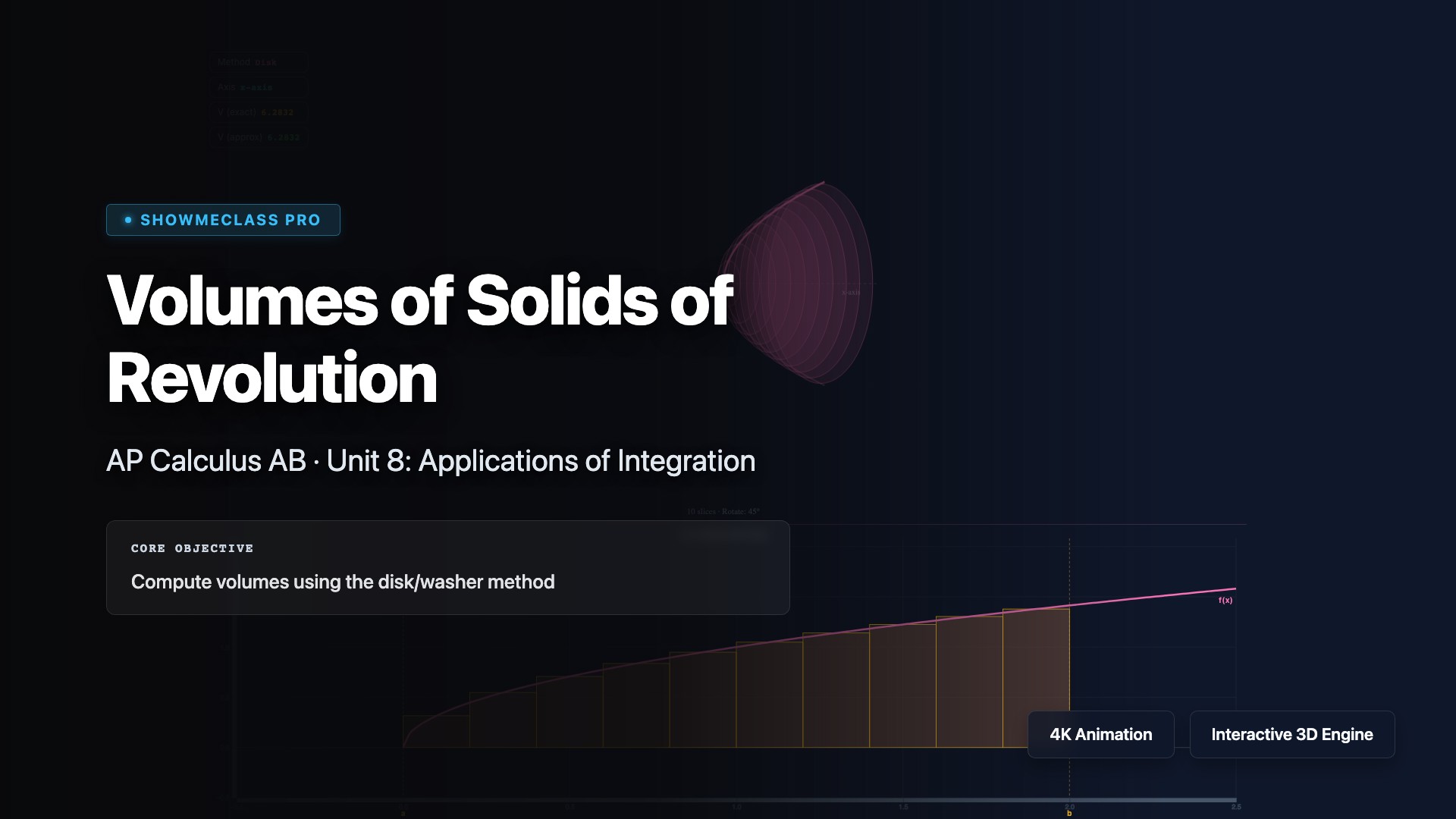
Volumes of Solids of Revolution
Calculate volumes of three-dimensional solids formed by rotating regions around axes using disk, washer, and shell methods. Visualize the disk method V = π∫[a to b] [R(x)]²dx for solids without holes, the washer method V = π∫[a to b] ([R(x)]² - [r(x)]²)dx for solids with holes, and the shell method V = 2π∫[a to b] x·h(x)dx for rotation around vertical axes. Master choosing the most efficient method for each problem.
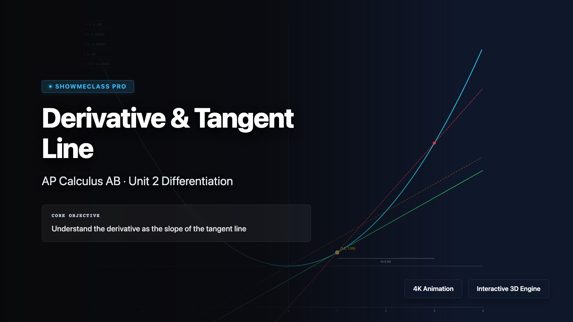
Derivative & Tangent Line Visualizer
Drag a point along any differentiable function to see the tangent line update in real time. Visualize how the slope of the tangent equals the derivative value, and explore where derivatives are zero or undefined.
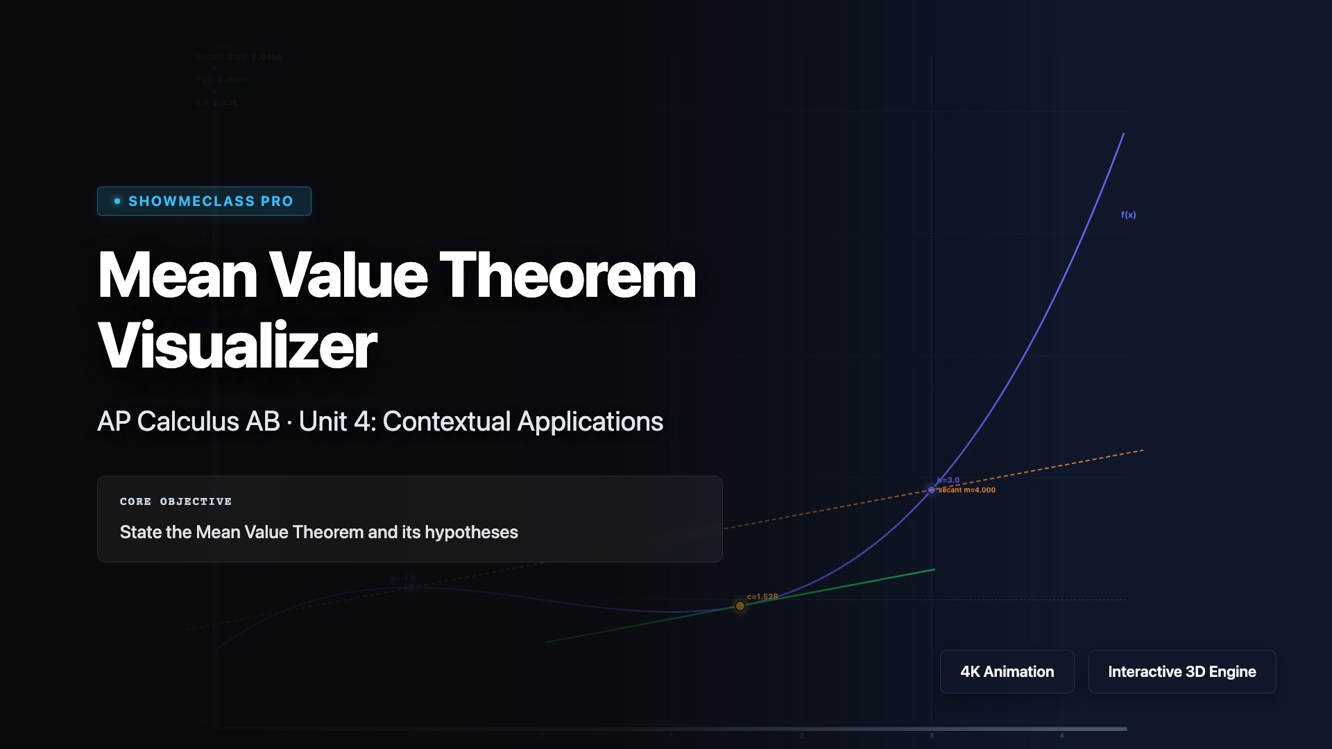
Mean Value Theorem Visualizer
Visualize the Mean Value Theorem (MVT), which guarantees that for a continuous and differentiable function on [a,b], there exists at least one point c where f'(c) = (f(b)-f(a))/(b-a). Explore how the instantaneous rate of change equals the average rate of change at some interior point. Understand MVT's applications in proving inequalities, analyzing motion, and establishing fundamental results like the constant difference theorem.
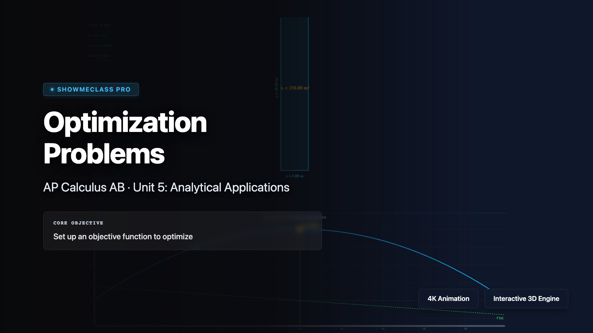
Optimization Problems
Solve optimization problems by finding absolute and relative extrema using calculus techniques. Learn to identify constraints, write objective functions, take derivatives, find critical points using f'(x) = 0, and apply the first or second derivative test. Explore real-world applications including maximizing area, minimizing cost, optimizing volume, and finding shortest distances in geometry, physics, and economics.
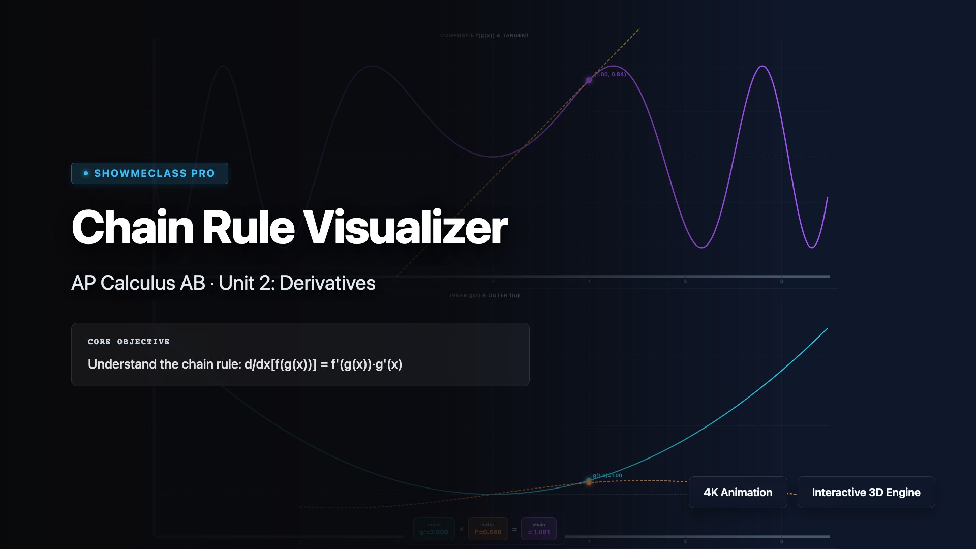
Chain Rule Visualizer
Visualize the chain rule for differentiating composite functions, one of the most powerful differentiation techniques in calculus. Explore how d/dx[f(g(x))] = f'(g(x)) · g'(x) by decomposing nested functions into outer and inner components. Practice identifying composite functions, applying the chain rule step-by-step, and understanding how rates of change multiply through function composition.
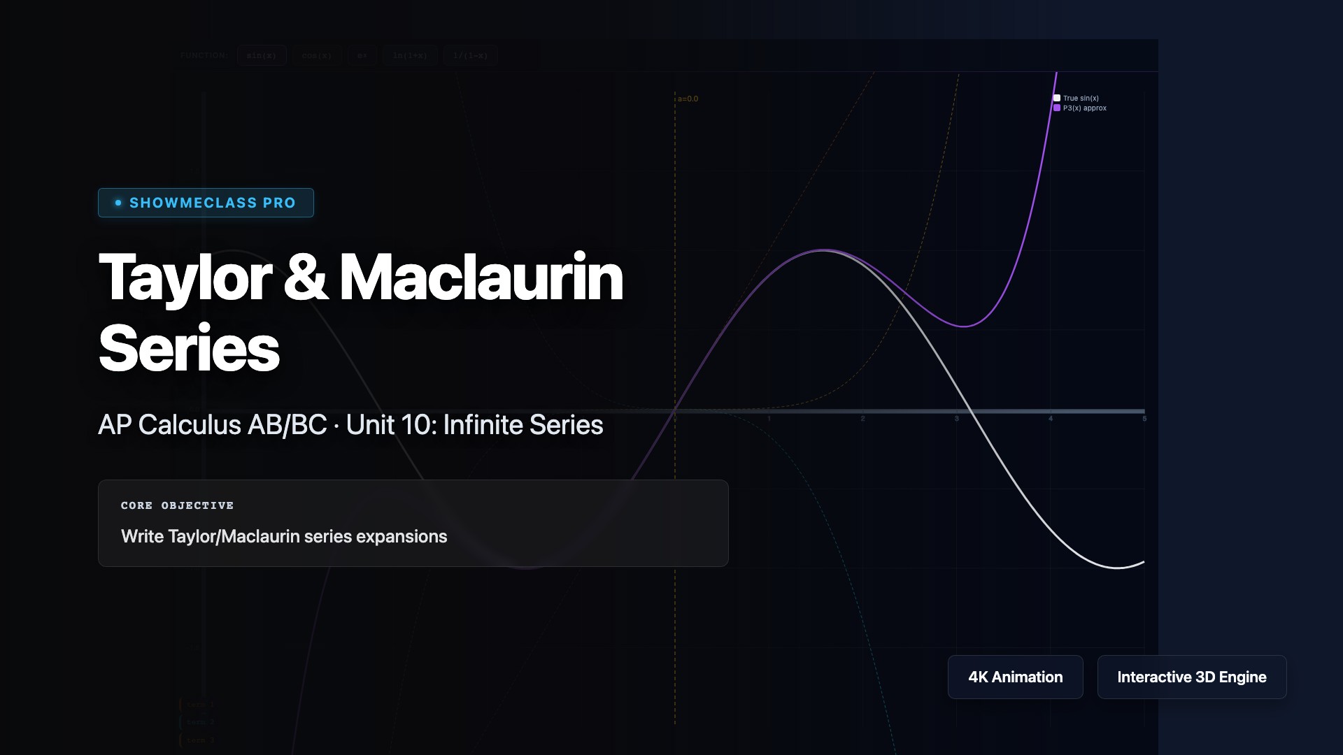
Taylor Series
Explore Taylor and Maclaurin series, which approximate functions as infinite polynomials using derivatives at a single point. Visualize how f(x) ≈ f(a) + f'(a)(x-a) + f''(a)(x-a)²/2! + ... converges to the original function. Understand how adding more terms improves accuracy, and learn common series for e^x, sin(x), cos(x), and ln(1+x). Practice finding intervals of convergence and estimating error bounds.
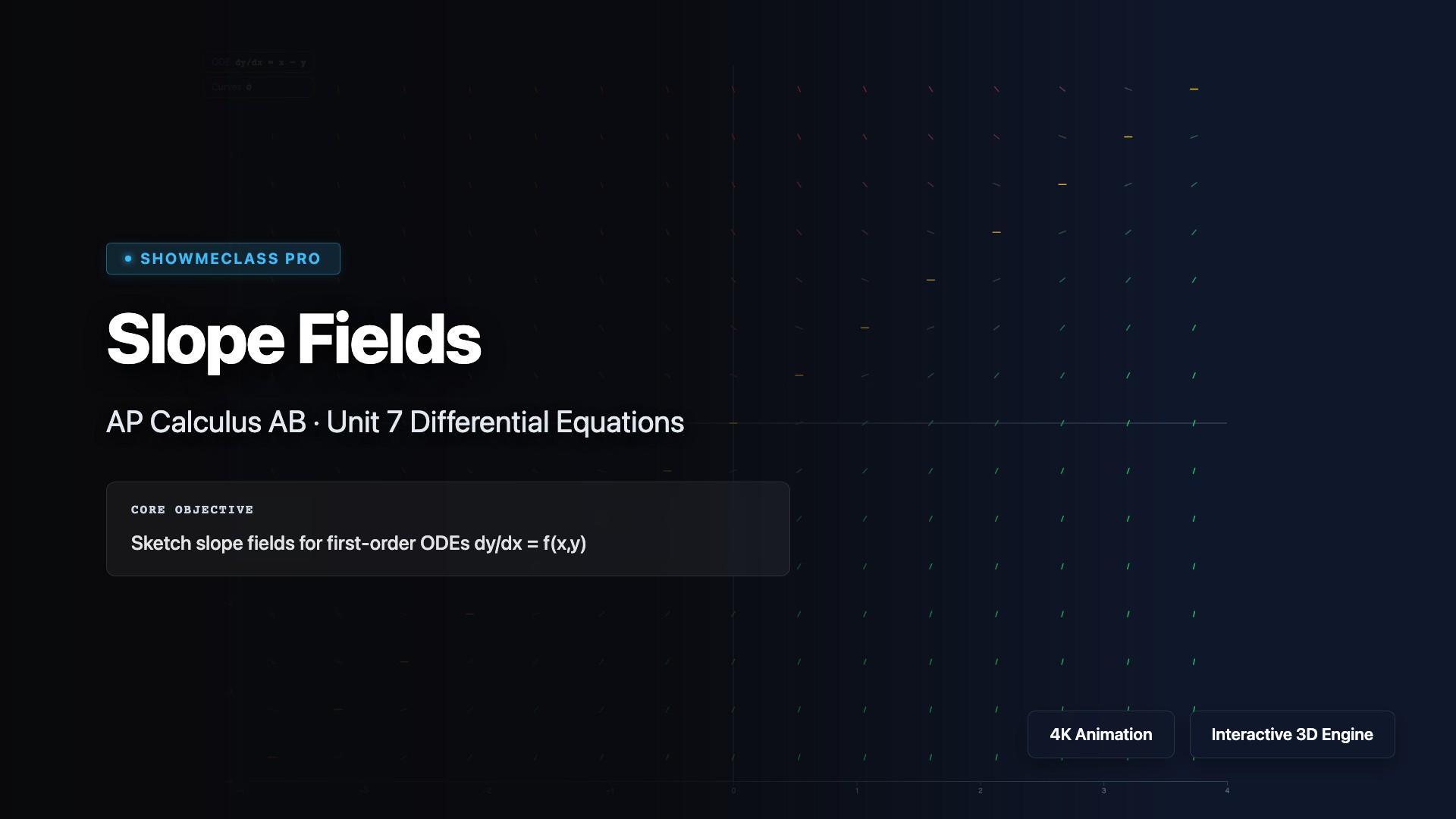
Slope Field Explorer
Generate slope fields for any first-order ODE and trace solution curves through arbitrary initial conditions. Visualize how solutions behave near equilibria, and develop intuition for qualitative analysis.
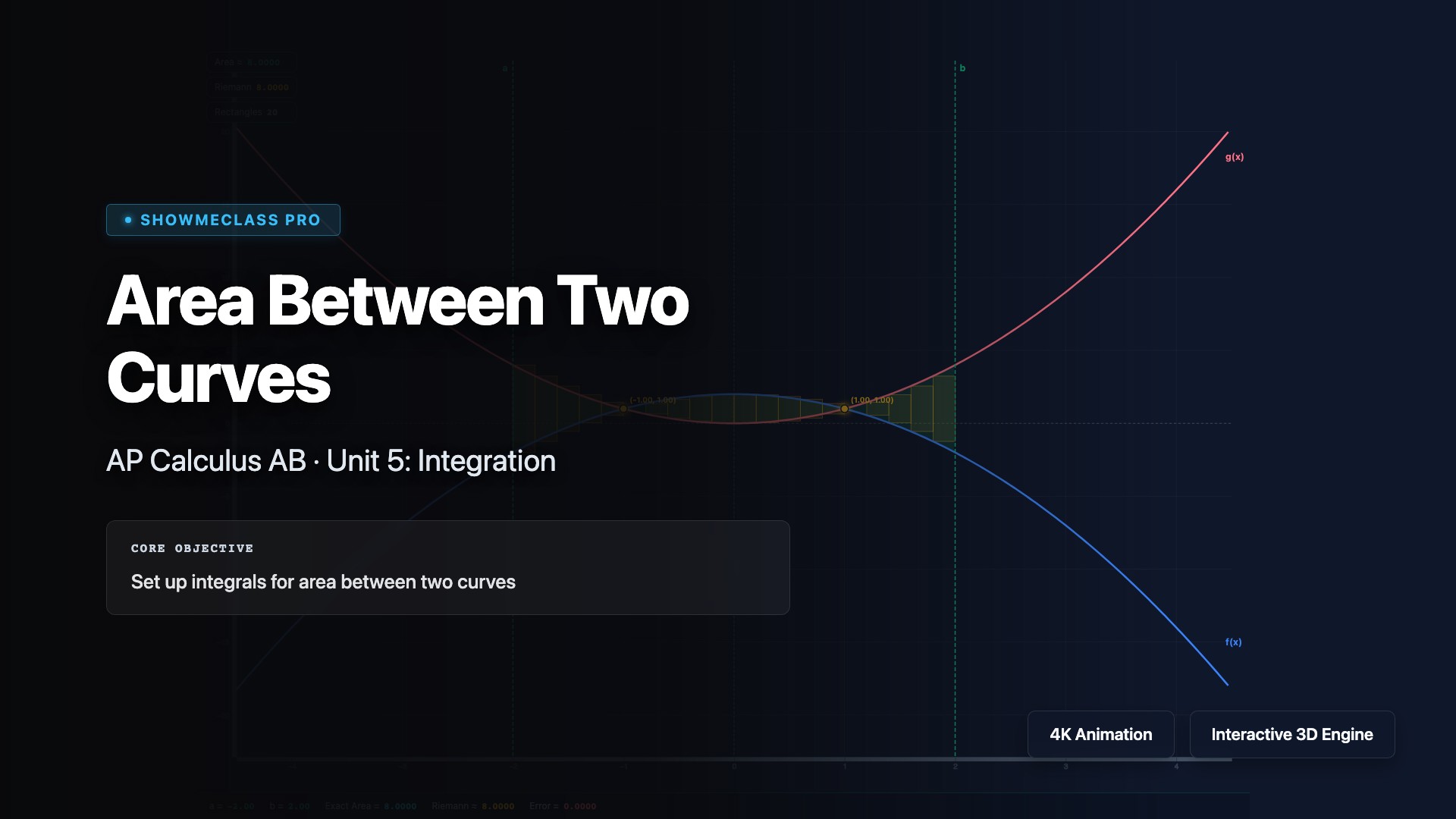
Area Between Two Curves
Visualize and calculate the area between two curves using definite integrals. Explore how to find intersection points, determine which function is on top, and set up the integral ∫[a to b] (f(x) - g(x))dx. Practice with vertical and horizontal slicing methods, and understand applications in physics, economics, and geometry where finding regions between curves is essential.
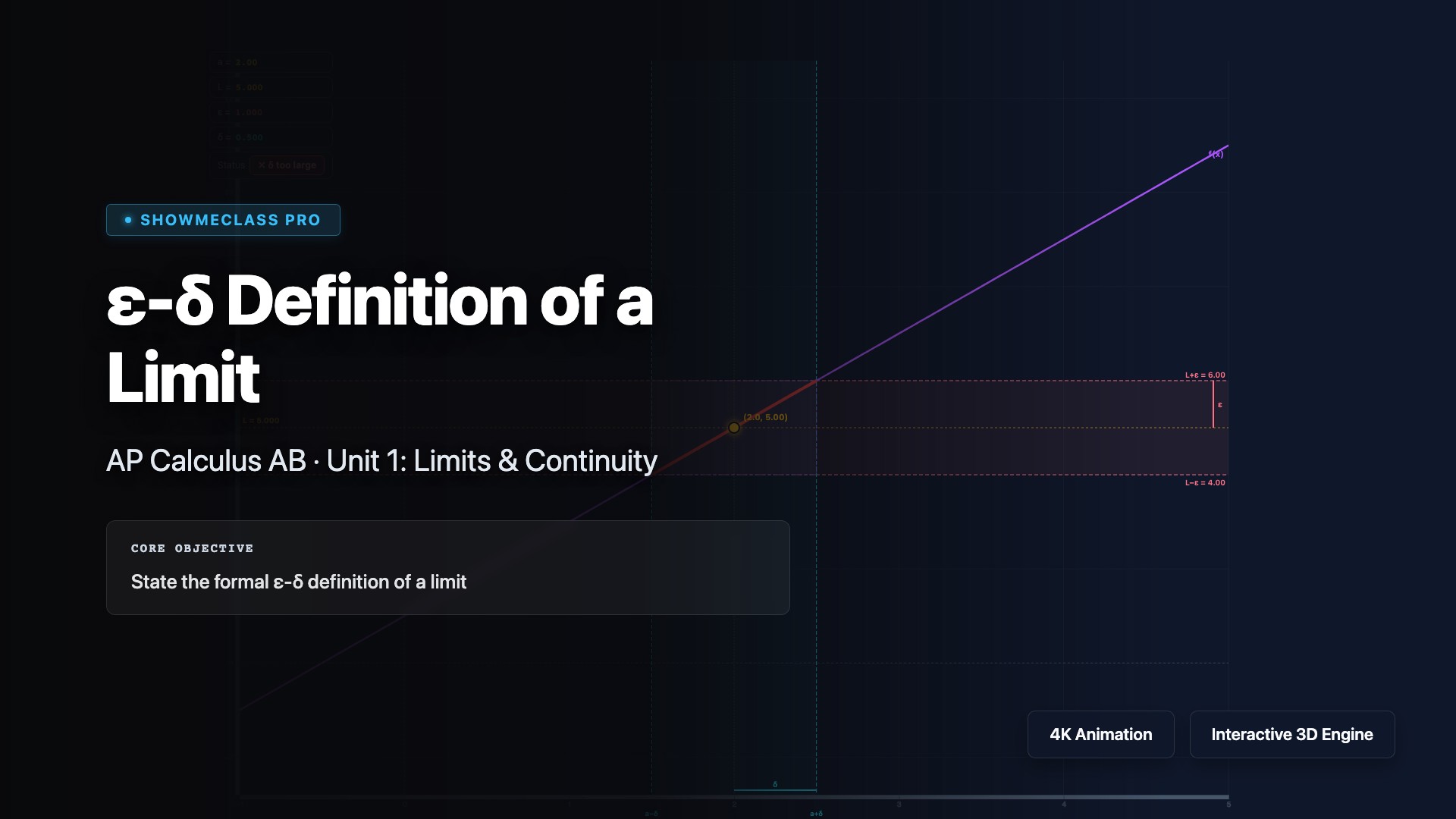
ε-δ Definition of a Limit
Explore the rigorous epsilon-delta (ε-δ) definition of a limit, the formal foundation of calculus. Visualize how for every ε > 0, there exists a δ > 0 such that if 0 < |x - c| < δ, then |f(x) - L| < ε. Understand how this definition precisely captures the intuitive notion that f(x) approaches L as x approaches c, and practice constructing epsilon-delta proofs.
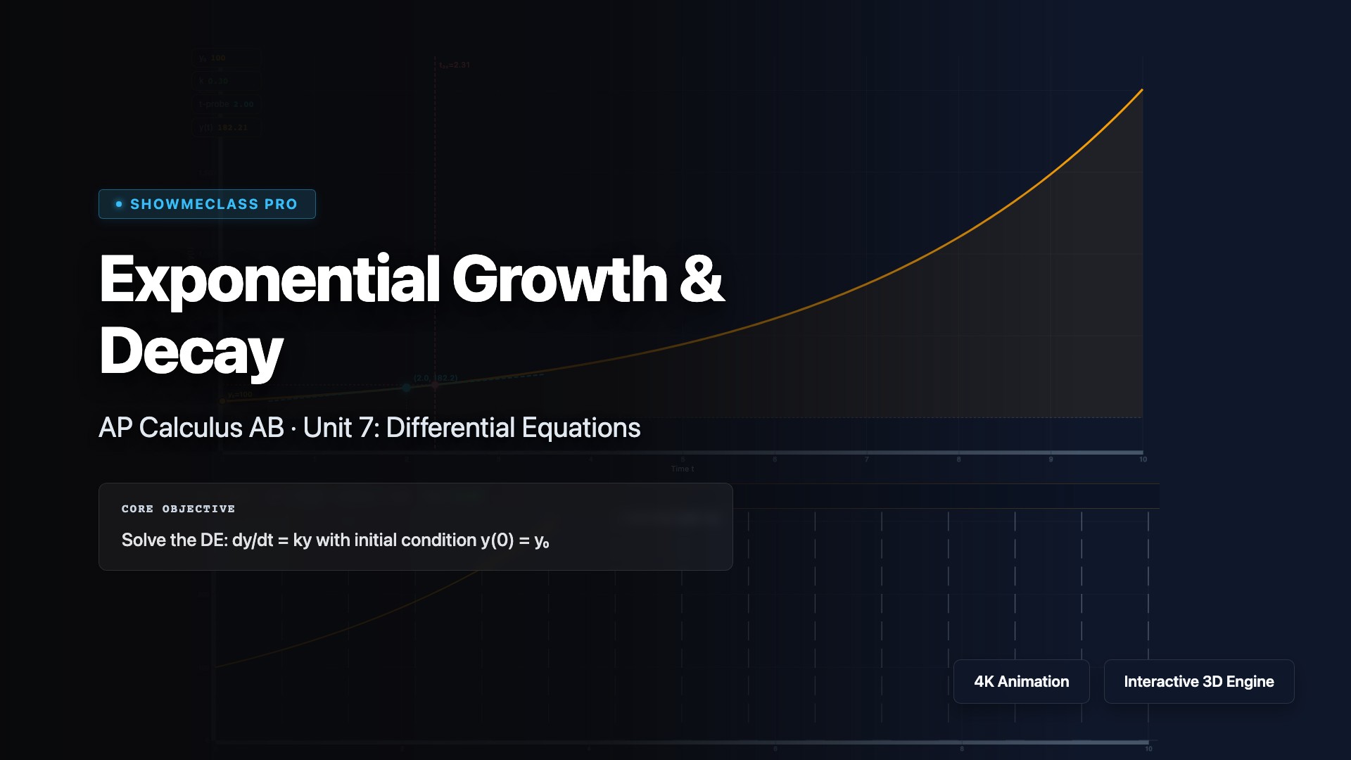
Exponential Growth & Decay
Model exponential growth and decay processes using differential equations of the form dy/dt = ky. Explore how the solution y = y₀e^(kt) describes phenomena like population growth, radioactive decay, compound interest, and Newton's law of cooling. Understand the significance of the growth constant k, half-life, and doubling time in real-world applications across biology, physics, and finance.
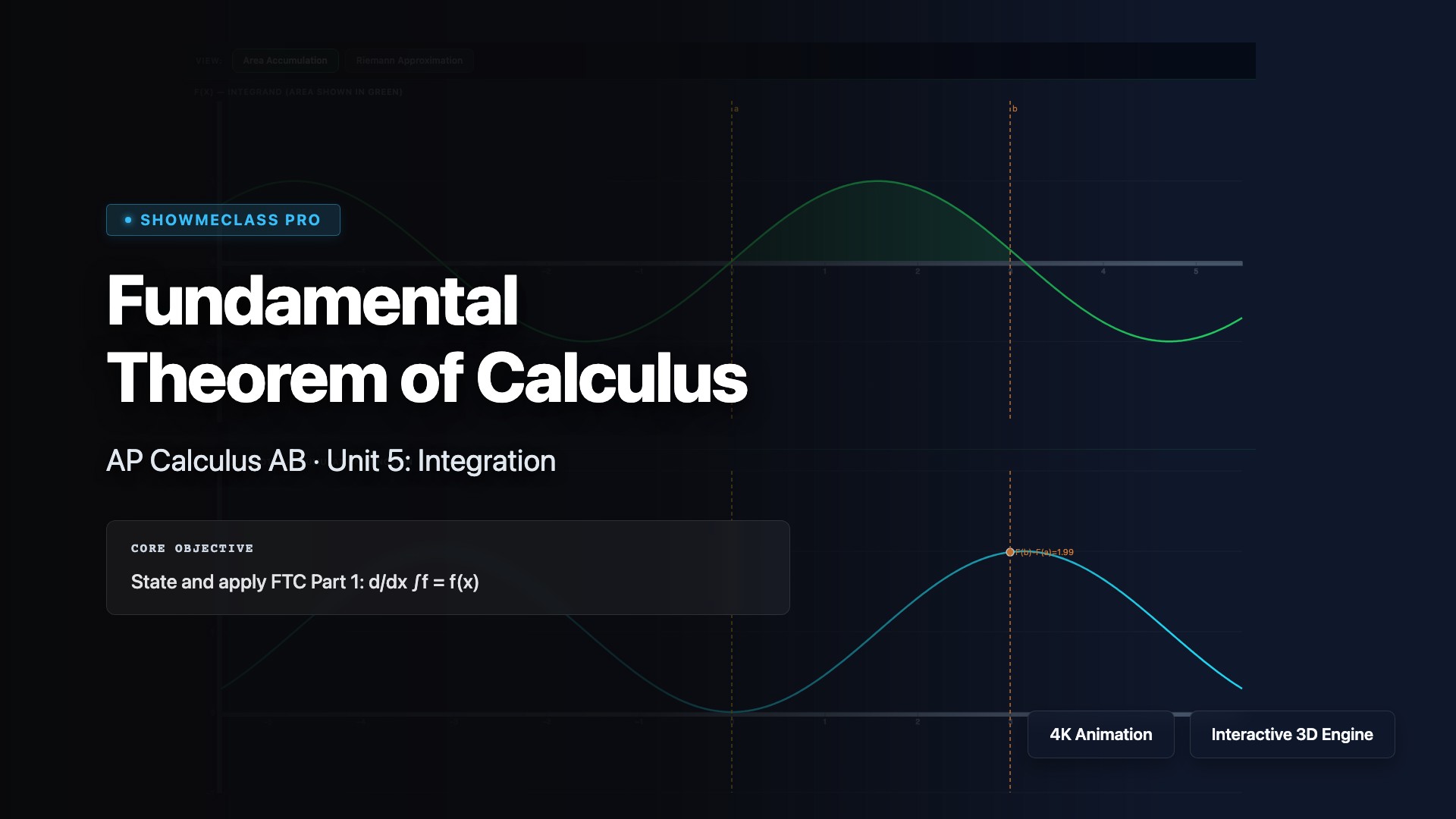
Fundamental Theorem of Calculus
Explore the Fundamental Theorem of Calculus, which connects differentiation and integration as inverse operations. Visualize Part 1: if F(x) = ∫[a to x] f(t)dt, then F'(x) = f(x), and Part 2: ∫[a to b] f(x)dx = F(b) - F(a) where F is any antiderivative of f. Understand how this theorem enables efficient calculation of definite integrals and reveals the deep relationship between rates of change and accumulation.

Volumes w/ Known Cross Sections
Calculate volumes of solids with known cross-sectional shapes perpendicular to an axis using integration. Visualize how V = ∫[a to b] A(x)dx sums infinitely many cross-sectional areas—squares, rectangles, semicircles, equilateral triangles, and isosceles right triangles. Understand how the base region determines the limits of integration and how the cross-section shape determines the area function A(x).
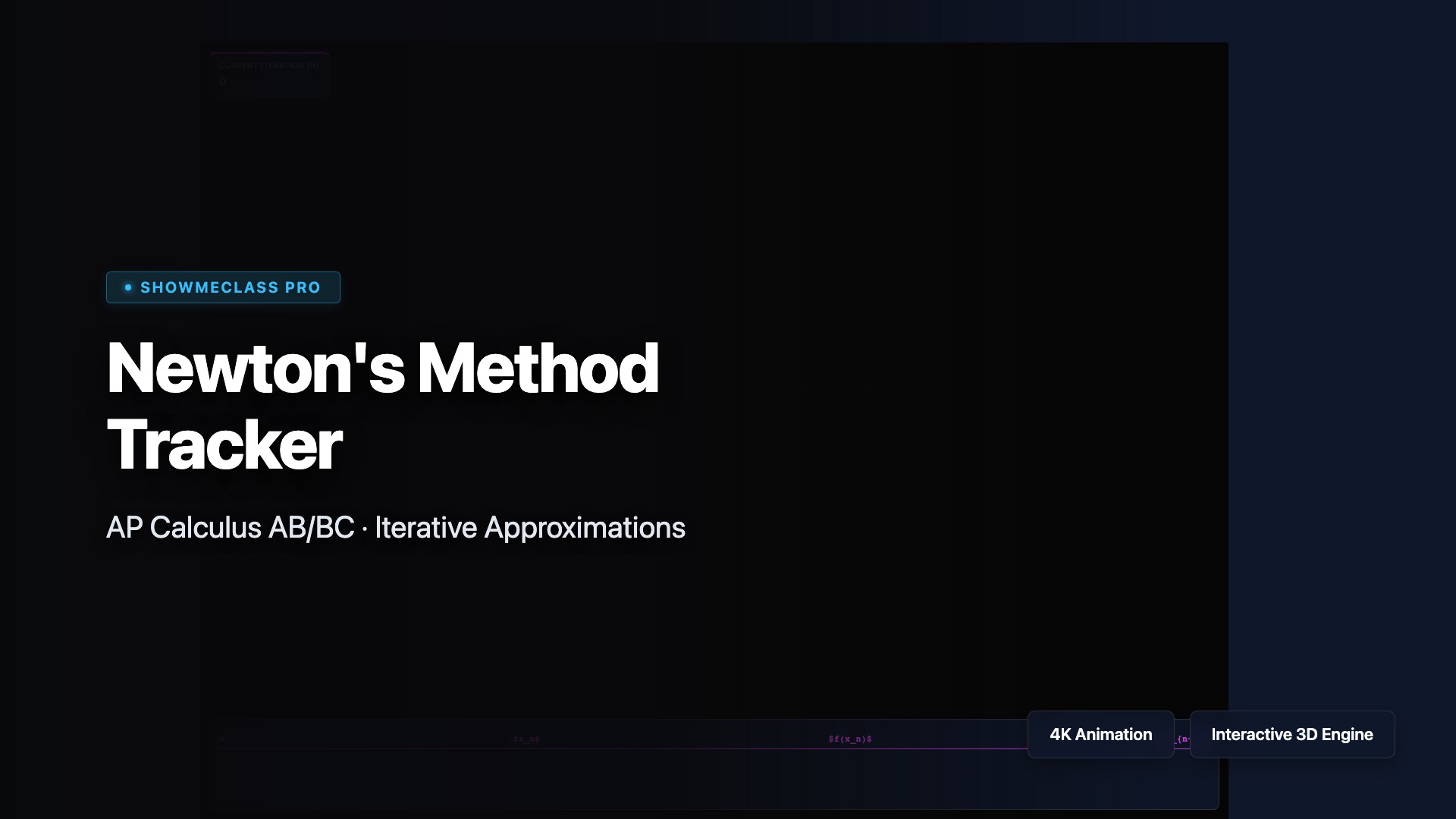
Newton-Raphson Method Root Finder
Track the wild convergence of Newton's Method. Place an initial guess x0 and watch iterative tangent lines slice toward the true polynomial root. Place the guess at a local minimum (f'(x)=0) to provoke absolute visual divergence.
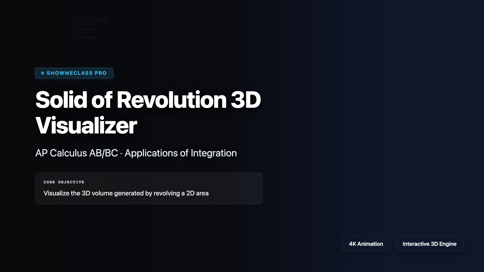
Solid of Revolution 3D Visualizer
Interactive Calculus visualizer converting 2D function areas into 3D volumes of revolution using Disk and Washer methods.

Limits & Continuity Explorer
Interactive limit evaluation (left-hand, right-hand, absolute) and 3-step continuity logical check tool simulating removable, jump, infinite, and oscillating discontinuities.
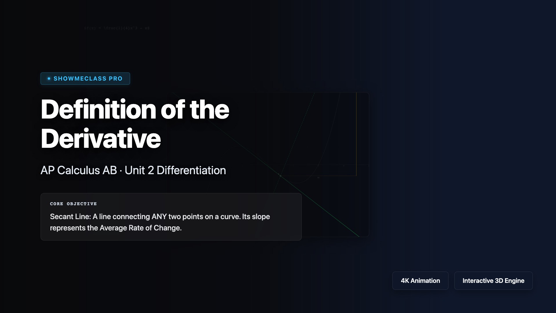
Definition of the Derivative
Interactive secant-to-tangent limit convergence visualizing the formal definition of the derivative with dynamic dx collapsing.
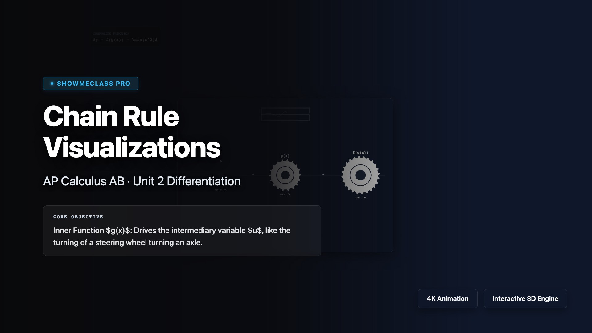
Chain Rule Visualizations
Mechanical gear visualization translating the abstract composite derivative multiplication f'(g(x)) * g'(x) into physical rotational interlocking.
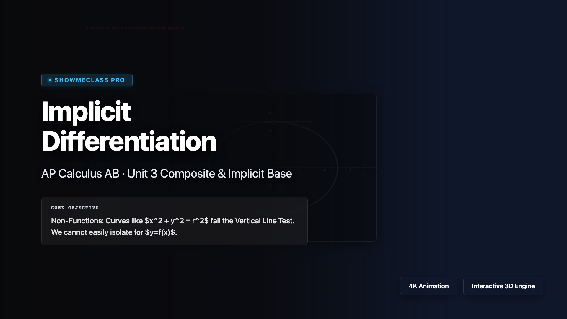
Implicit Differentiation
Implicit differentiation analyzer for non-functions (Circles, Ellipses, Foliums). Evaluates dy/dx dynamically, reacting to both x and y inputs to map vertical and horizontal tangents.
Related Rates Visualizer
Related rates visualization using implicit chain rule integration with respect to time (dt). Demonstrates the geometric parameter shift paradox of Constant dV/dt impacting spherical radii and conical fill heights dynamically.

MVT & Rolle's Explorer
MVT interactive module letting users sweep endpoints to compute the secant, subsequently automatically identifying all internal $c$ points where tangent perfectly parallels secant. Built with Rolle's edge case and cusp logic breakers.

Riemann Sum Approx
Interactive summation explorer comparing Left, Right, Midpoint Riemann sums and Trapezoidal logic. N-slider rapidly expands bounding box series $\Sigma$ into exact integral space via $N \rightarrow \infty$, dynamically revealing errors algebraically and geometrically.
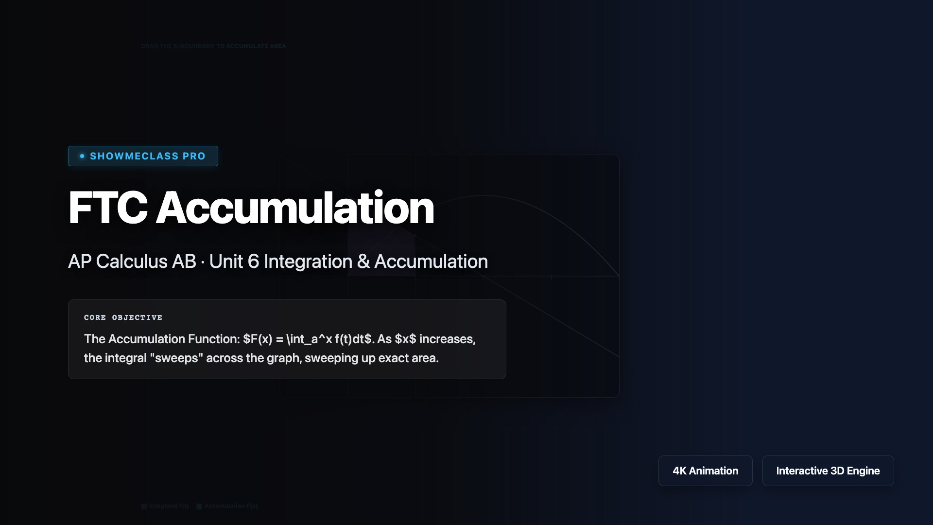
FTC Accumulation
Fundamental Theorem of Calculus visually represented. Sweeps across $f(t)$ bounds bridging dynamic differential area accumulation natively into the $F(x)$ graphing engine.
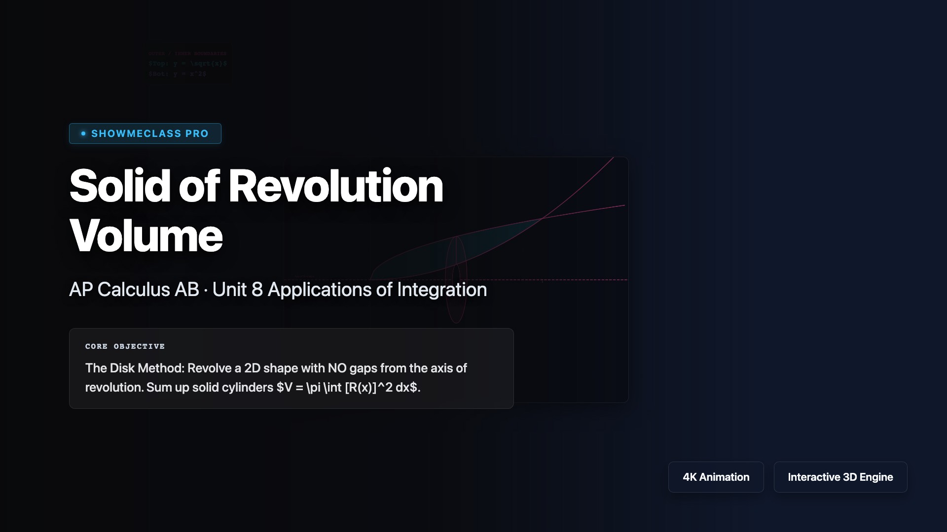
Solid of Revolution Volume
Volumetric solids of revolution visualizer computing the Washer Method natively via integral bounds. Calculates both standard axis limits and offset axis shifts dynamically.

Slope Field Explorer
Slope field generator plotting directional isoclines. Includes an interactive differential Euler-trace mechanism resolving specific math solutions when a distinct Initial Condition point is dropped onto the coordinate grid.
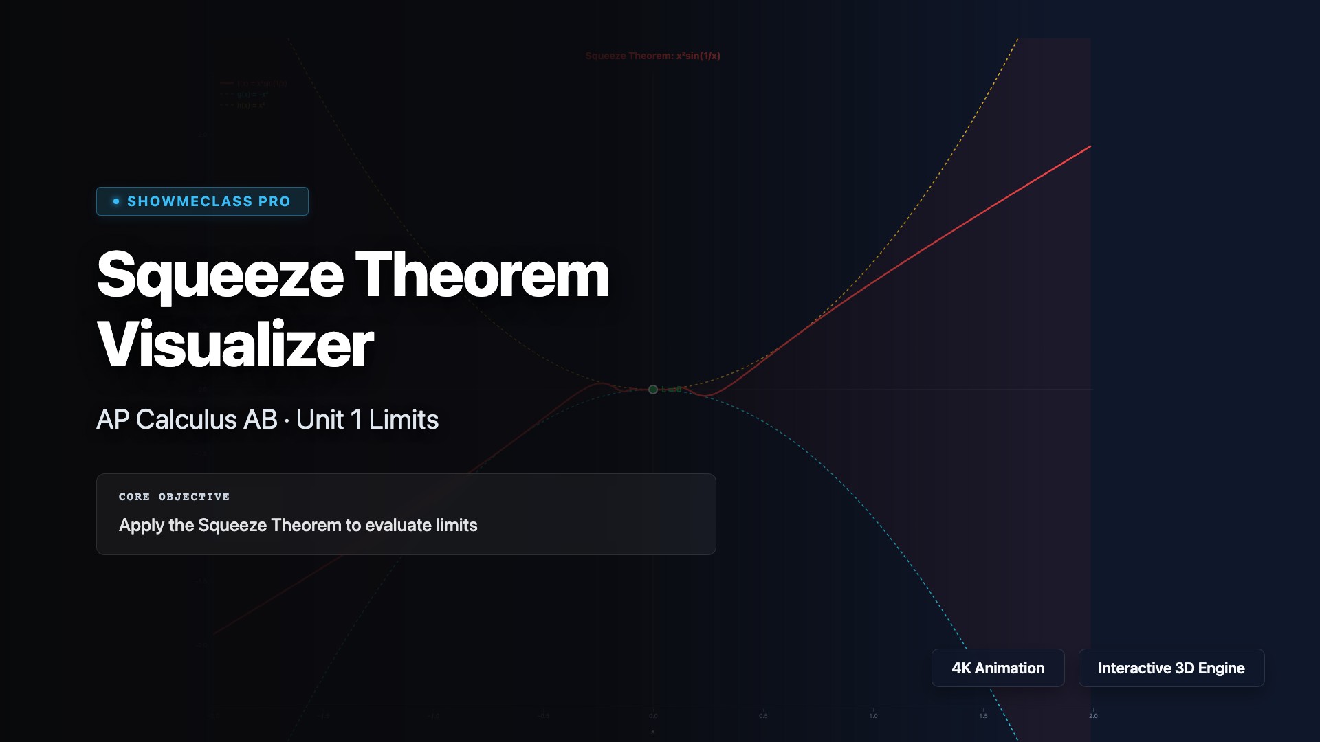
Squeeze Theorem Visualizer
Interactive visualization of the Squeeze Theorem with 4 classic examples (x²sin(1/x), sin(x)/x, x·cos(1/x), (1−cos x)/x²). Shows bounding functions g(x) ≤ f(x) ≤ h(x) with shaded squeeze region. Adjustable zoom and convergence to limit point.
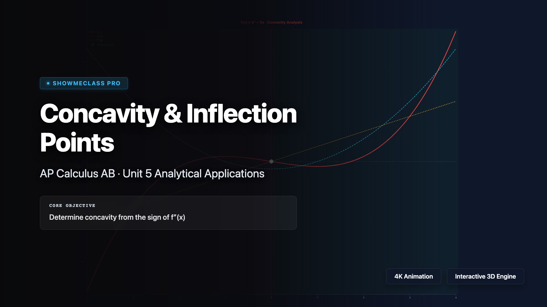
Concavity & Inflection Points
Interactive concavity analysis showing f(x), f′(x), and f″(x) simultaneously for 4 functions. Concavity shading (green=up, red=down), inflection point markers, and movable cursor with real-time derivative values and concavity classification.
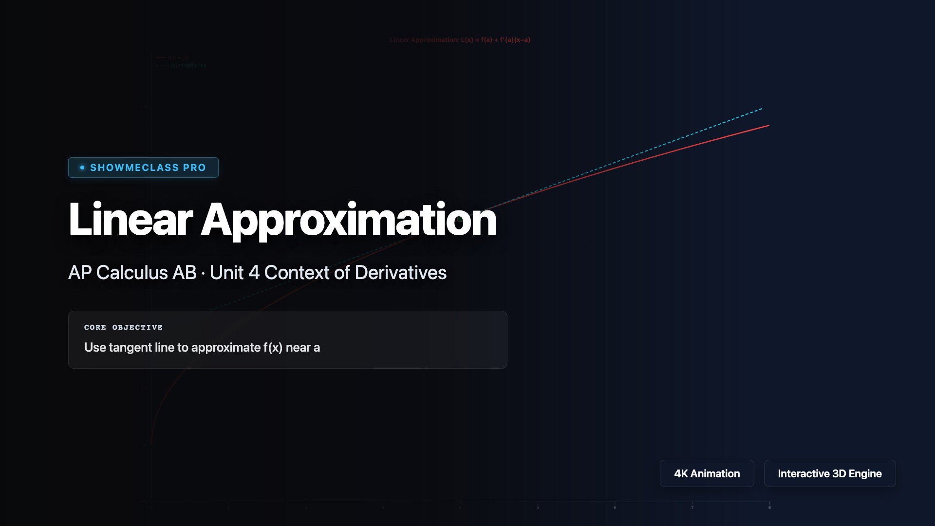
Linear Approximation & Differentials
Interactive linearization visualizer for 5 functions (√x, sin(x), eˣ, ln(x), 1/(1+x)). Shows tangent line L(x) = f(a) + f′(a)(x−a) overlaid on actual curve. Movable x-cursor with real-time exact vs approximate values, absolute and percentage error calculation.

u-Substitution Step-by-Step
Step-by-step walkthrough of u-substitution for 6 integral examples. Color-coded steps: identify u, find du, match dx, substitute, integrate, back-substitute. Covers standard patterns including definite integrals with bound conversion.
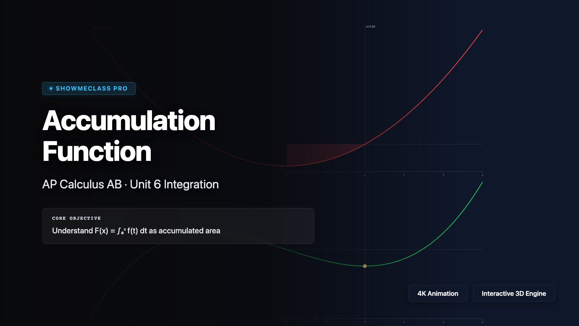
Accumulation Function Visualizer
Dual-panel visualization of f(t) and F(x) = ∫ₐˣ f(t) dt. Shows signed area shading (green positive, red negative) on the integrand graph alongside the accumulation function. Demonstrates FTC Part 1: F′(x) = f(x). Adjustable upper limit x with 4 function examples.

Separable Differential Equations
Slope field visualization with Euler method solution curves for 4 classic separable ODEs (dy/dx=xy, −y/x, y(1−y) logistic, x/y). Adjustable initial condition y₀ with multiple solution curves. Step-by-step separation and integration displayed.
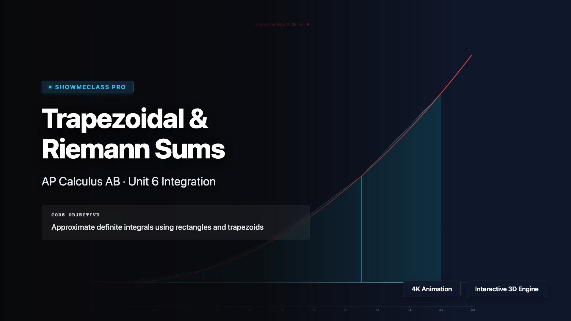
Trapezoidal & Riemann Sum Approximation
Interactive numerical integration comparing Left, Right, Midpoint, and Trapezoidal rules. 4 functions with adjustable number of subintervals (n=1 to 50). Shows exact value, approximation, absolute and percentage error. Visualizes rectangles/trapezoids overlaid on curve.
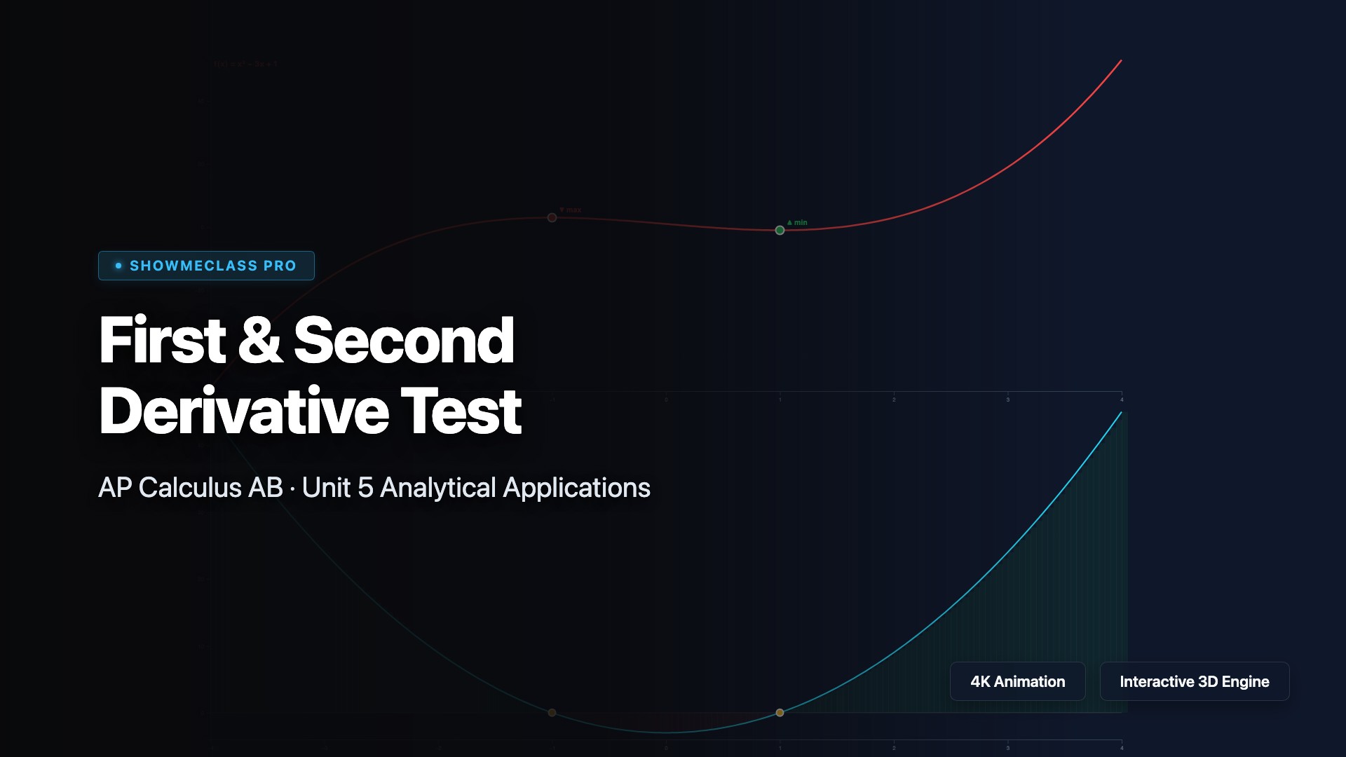
First & Second Derivative Test
Dual-panel display of f(x) and f′(x) for 4 polynomial/exponential functions. Critical points marked with max/min labels, f′ sign shading (green=increasing, red=decreasing). Second derivative test verification at each critical point. Interactive function selection.
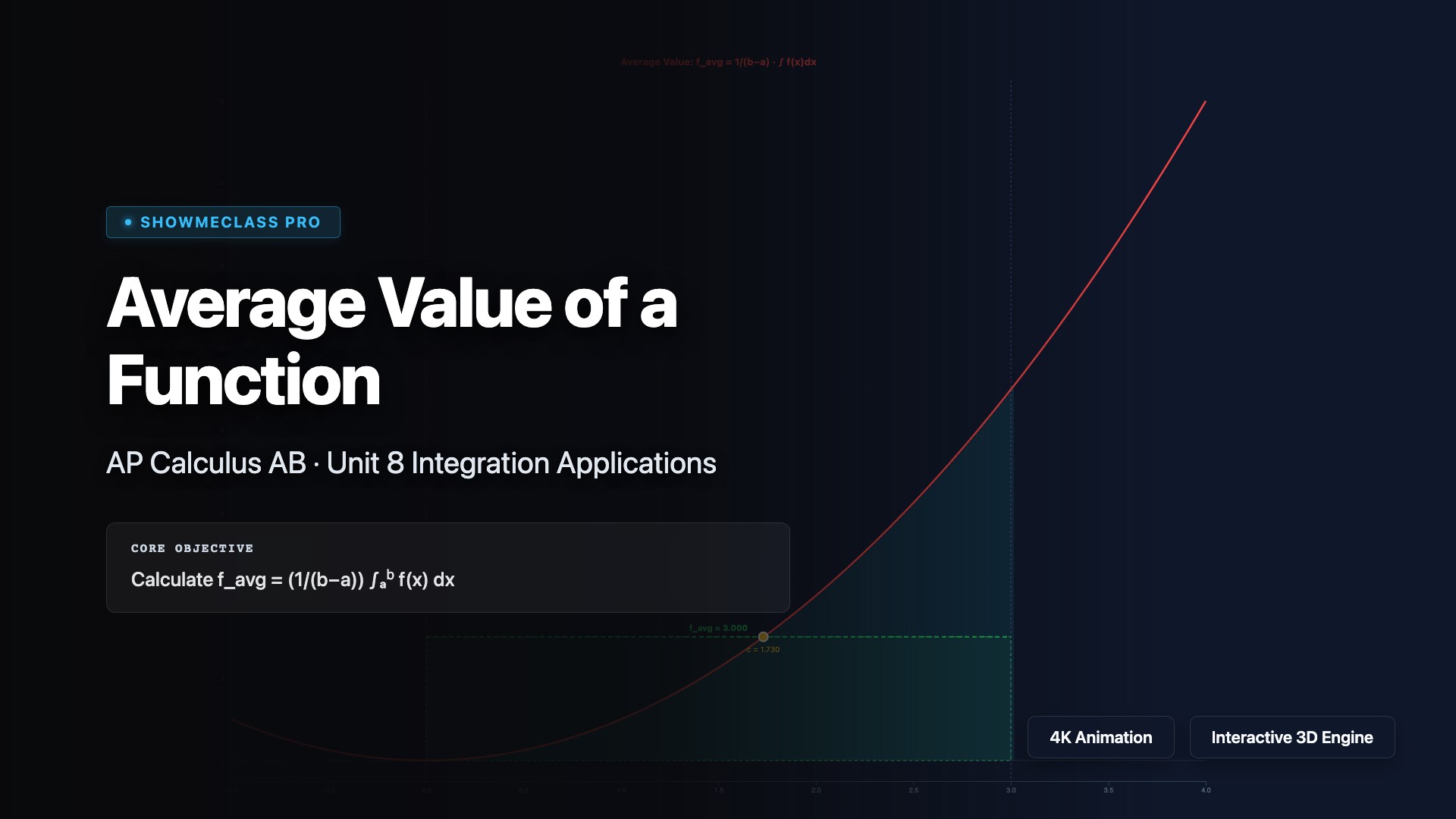
Average Value of a Function
Interactive average value calculator showing f_avg = 1/(b−a)·∫f(x)dx with equal-area rectangle visualization. Green dashed line at f_avg height creates a rectangle with the same area as the integral. Finds MVT for Integrals c-value. Adjustable bounds a and b.