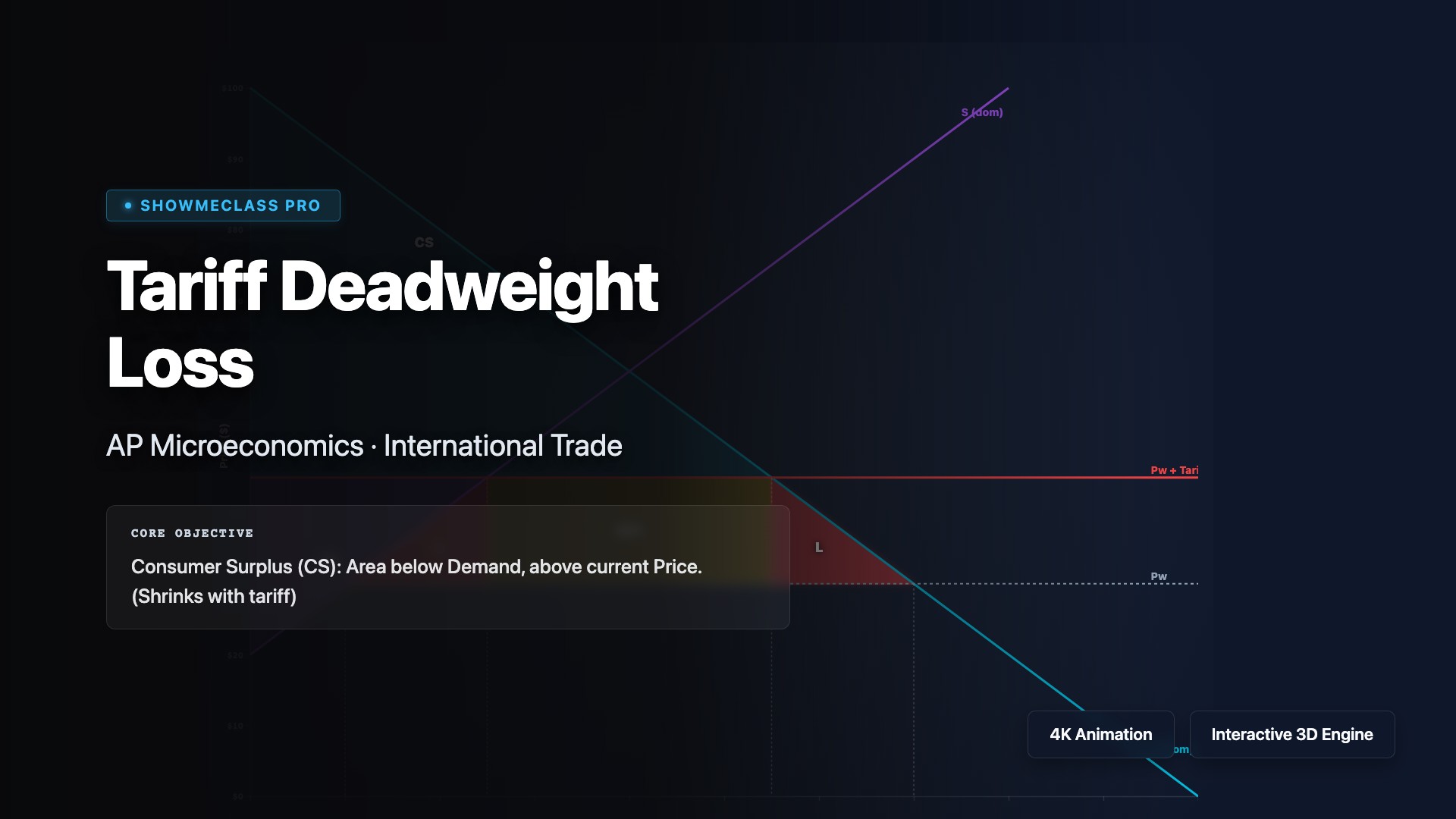
Tariff Deadweight Loss
Simulate protectionist trade policy. Imposing a tariff elevates the world price, mathematically shrinking Consumer Surplus while generating Government Revenue and Deadweight Loss triangles.

Profit Maximization (MR = MC)
Drag the market price line to find the optimal quantity where MR intercepts Marginal Cost. Instantly calculates Total Economic Profit or identifies the Shutdown point when Price falls below AVC.

LRATC Envelope Curve
Understand firm costs in the Long Run. Slide targeted production scales to track how Short-Run Average Total Cost curves (SRATC) form the Returns to Scale envelope.

Lorenz Curve & Gini
Graph income inequality mathematically. Bend the Lorenz curve from Perfect Equality to extreme inequality and watch the Gini Coefficient (A/(A+B)) update in real-time.

Game Theory Payoff Matrix
Model oligopolistic behavior. Highlights Dominant Strategies and Best Responses to isolate Nash Equilibriums in classic scenarios.

Production Possibilities Frontier
Explore the Production Possibilities Frontier (PPF) curve showing the maximum combinations of two goods an economy can produce with limited resources. Understand opportunity cost (the slope of the PPF), efficiency (points on the curve), inefficiency (points inside), and impossibility (points outside). Visualize how economic growth shifts the PPF outward, and how the law of increasing opportunity costs creates the bowed-out shape as resources are reallocated.

Market Structures Comparison
Compare the four market structures: perfect competition (many firms, identical products, price takers), monopolistic competition (many firms, differentiated products, some price control), oligopoly (few firms, interdependent decisions, strategic behavior), and monopoly (single firm, unique product, price maker). Understand how each structure determines pricing using MR=MC, barriers to entry, long-run economic profit, and efficiency outcomes for consumers and society.

Supply & Demand Curves
Visualize supply and demand curves intersecting at market equilibrium where quantity supplied equals quantity demanded. Explore the law of demand (inverse price-quantity relationship) and law of supply (direct price-quantity relationship). Understand how shifts in demand (income, preferences, related goods) or supply (input costs, technology, expectations) create shortages or surpluses that drive price adjustments back to equilibrium. Practice analyzing how market forces allocate scarce resources efficiently.

Price Elasticity of Demand
Analyze price elasticity of demand (PED) measuring how quantity demanded responds to price changes using the formula %ΔQd / %ΔP. Classify demand as elastic (|PED| > 1, price changes significantly affect quantity), inelastic (|PED| < 1, quantity relatively unresponsive), or unit elastic (|PED| = 1). Understand how elasticity affects total revenue: price increases raise revenue for inelastic goods but lower revenue for elastic goods. Explore determinants including substitutes, necessity, and time horizon.

Price Controls & Surplus Visualizer
Impose brutal government administrative limits on the Free Market. Slide Price Ceilings (Rent Control) and Price Floors (Minimum Wage) across the equilibrium to instantly graphically calculate the resulting Shortage/Surplus and Deadweight Loss.

Tax Incidence & Deadweight Loss Simulator
Settle the debate over who actually pays taxes. Adjust Supply/Demand elasticities and apply an Excise Tax to instantaneously visualize the Consumer Burden (Blue), Producer Burden (Red), and the inefficient Deadweight Loss (Yellow).

Perfect Competition vs Monopoly
Compare the horizontal Demand curve of a Perfectly Competitive firm against the downward-sloping Demand curve of a Monopoly to locate Deadweight Loss (DWL).

Utility Maximization & Diminishing MU
Interactive total and marginal utility curves with diminishing returns bar chart. Adjust quantity and price to find consumer equilibrium where MU/P is optimized, with real-time consumer surplus calculation.

Indifference Curves & Budget Lines
Cobb-Douglas utility model showing indifference curves at multiple utility levels with adjustable budget constraint (income and prices). Visualizes optimal tangency point where MRS = price ratio for consumer equilibrium.

Factor Market (MRP = MRC)
Factor market labor hiring visualization where MRP = MR × MP declines due to diminishing marginal returns. Adjustable product price and wage rate reveal profit-maximizing employment level at MRP = MRC intersection.

Monopolistic Competition (SR/LR)
Monopolistic competition model showing differentiated product pricing with downward-sloping demand. Toggle between short-run profit, short-run loss, and long-run zero-profit tangency condition with ATC/MC/D/MR curves.

Oligopoly & Kinked Demand Curve
Kinked demand curve model explaining oligopoly price rigidity. Adjustable kink price and MC level demonstrate how the vertical MR gap allows cost changes without price adjustment — the core mechanism behind sticky prices in oligopolistic markets.