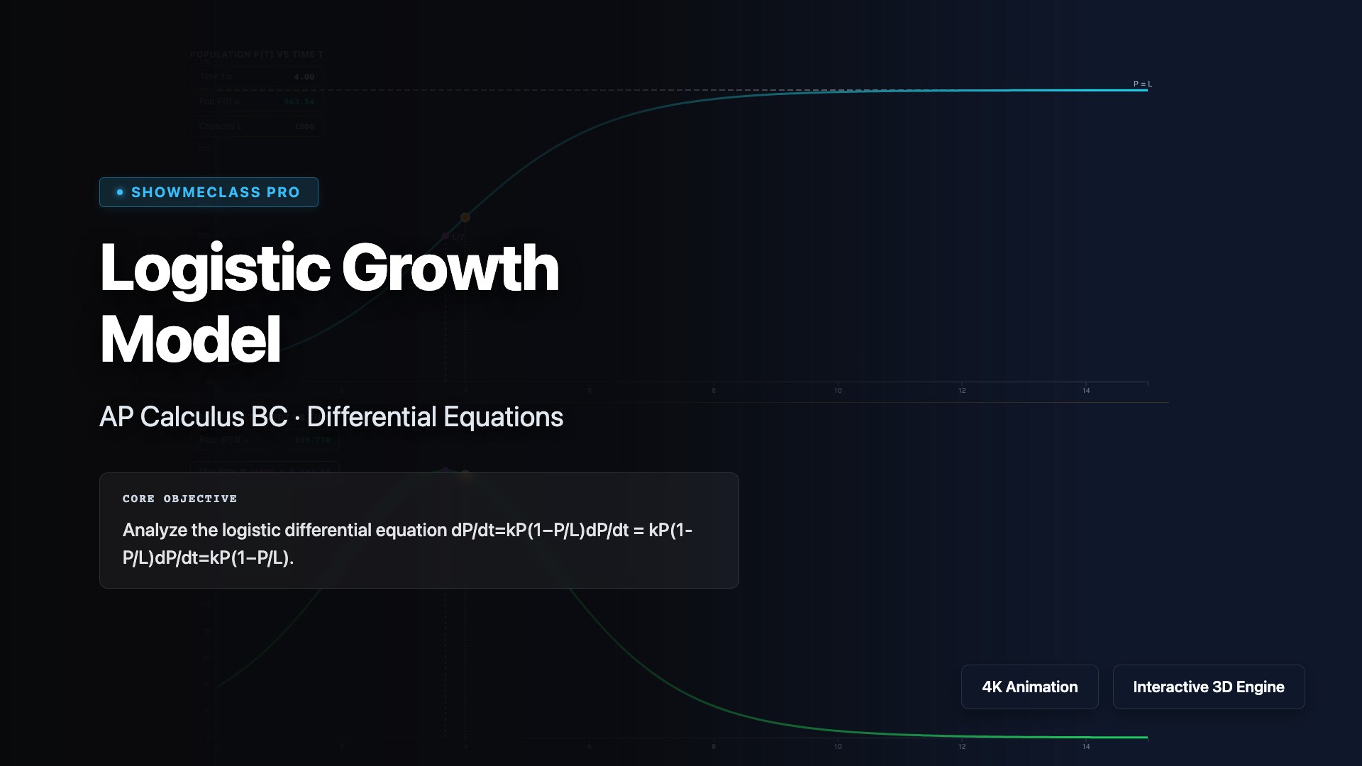
Logistic Growth Model
Model population growth with limited resources using the logistic differential equation dP/dt = kP(1 - P/M), where M is the carrying capacity. Visualize the S-shaped logistic curve P(t) = M/(1 + Ae^(-kt)) and understand how growth rate is fastest at P = M/2. Explore applications in ecology, epidemiology, and economics where growth is constrained by environmental factors, resource availability, or market saturation.
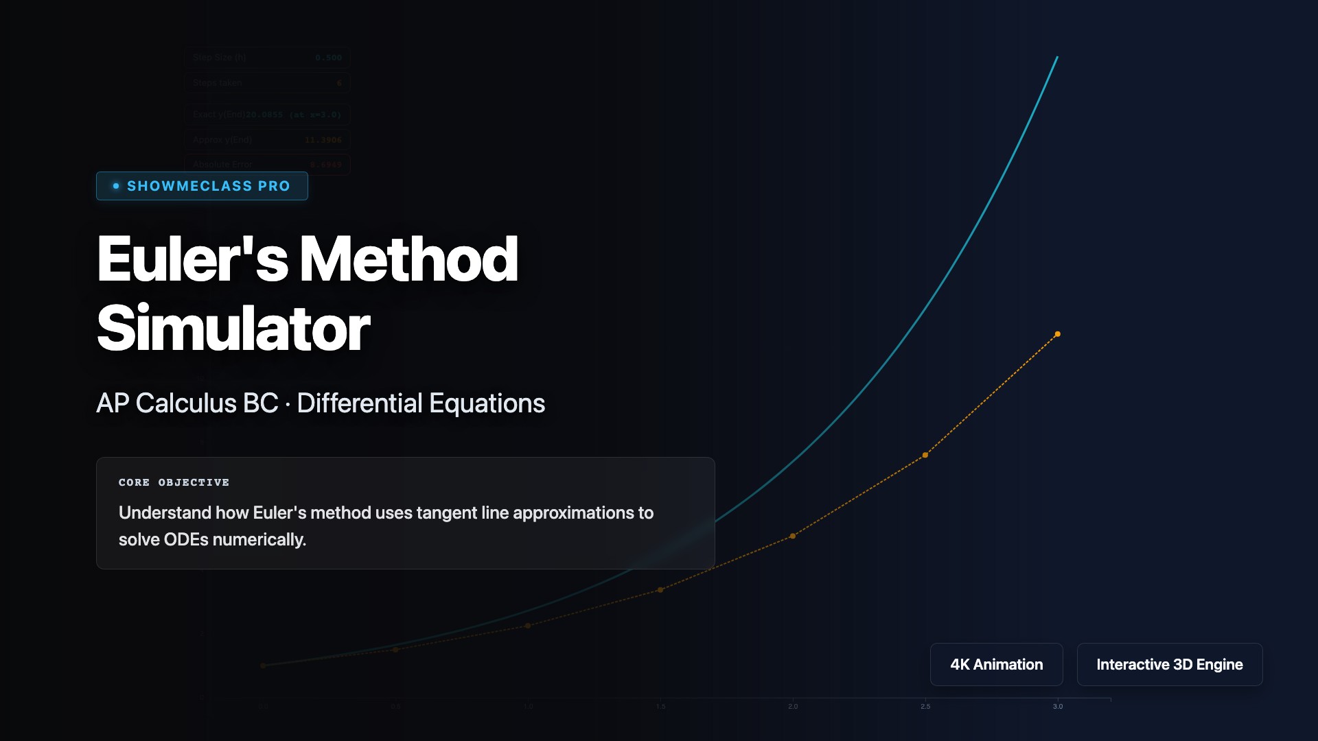
Euler's Method Simulator
Approximate solutions to differential equations using Euler's method, a numerical technique that uses tangent line approximations. Starting from an initial condition, iteratively calculate y_{n+1} = y_n + f(x_n, y_n)·Δx to trace the solution curve. Visualize how smaller step sizes improve accuracy, understand accumulation of error, and explore applications where analytical solutions are difficult or impossible to find.
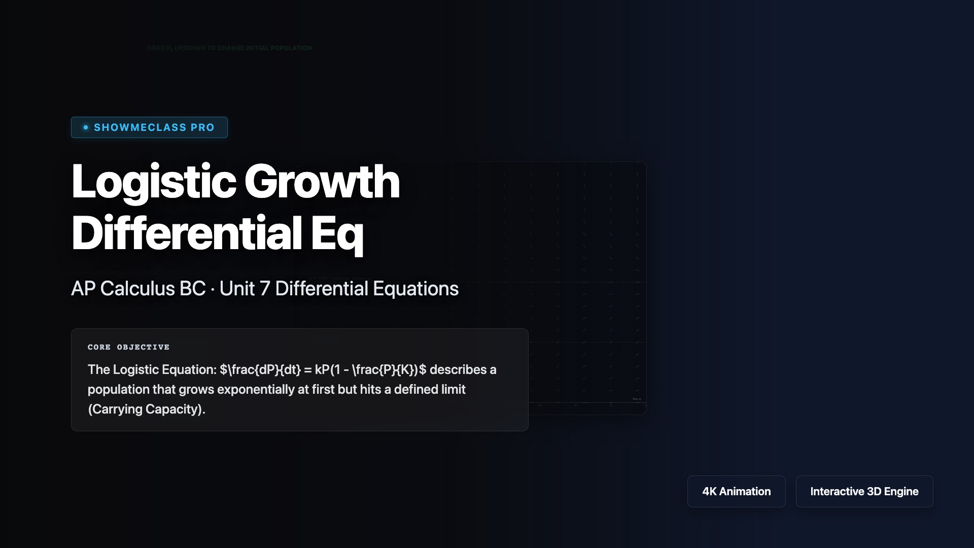
Logistic Growth Differential Eq
Differential logistic population map visualizing the $dP/dt = kP(1 - P/K)$ growth carrying capacity asymptote model. Sweeps dynamic background slopefields evaluating inflection velocity shifts mathematically derived from Partial Fractions.
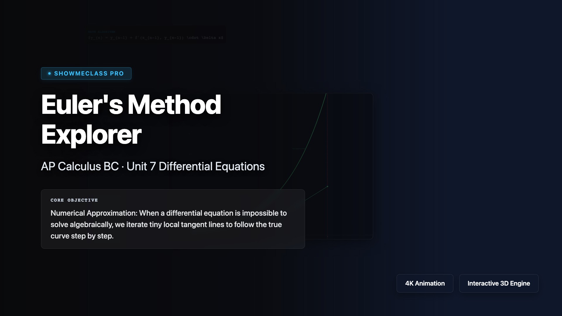
Euler's Method Explorer
Iterative numeric sequence plotting Euler's method vs True Analytical Solution paths. Modifying the $\Delta x$ subdivision actively updates truncation error margins mapping concave dynamics across polynomial and sinusoidal shift patterns.
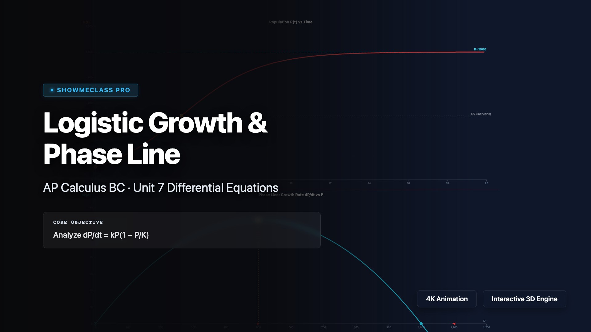
Logistic Growth & Phase Line
Dual-panel logistic differential equation analyzer. Top: P(t) solution curve with carrying capacity K and inflection at K/2. Bottom: dP/dt vs P parabolic phase space showing stable/unstable equilibria and maximum growth rate. Adjustable k, K, and P₀.