
Showing 12 results
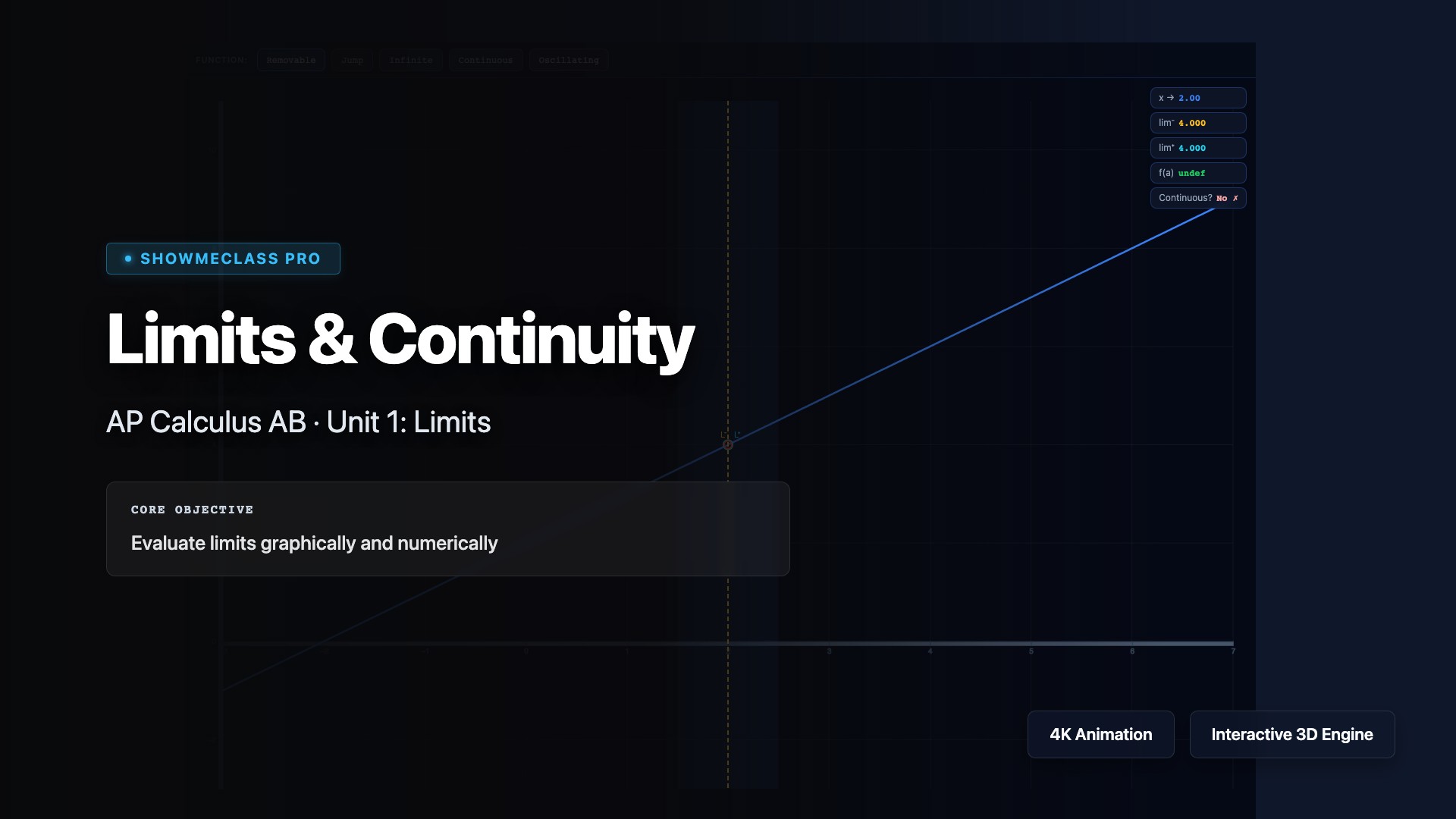
Limits & Continuity
Explore the foundational concepts of limits and continuity that underpin all of calculus. Visualize one-sided limits, two-sided limits, and limits at infinity. Understand the three conditions for continuity at a point: f(c) is defined, lim[x→c] f(x) exists, and lim[x→c] f(x) = f(c). Practice identifying discontinuities (removable, jump, and infinite) and applying limit laws to evaluate complex expressions.
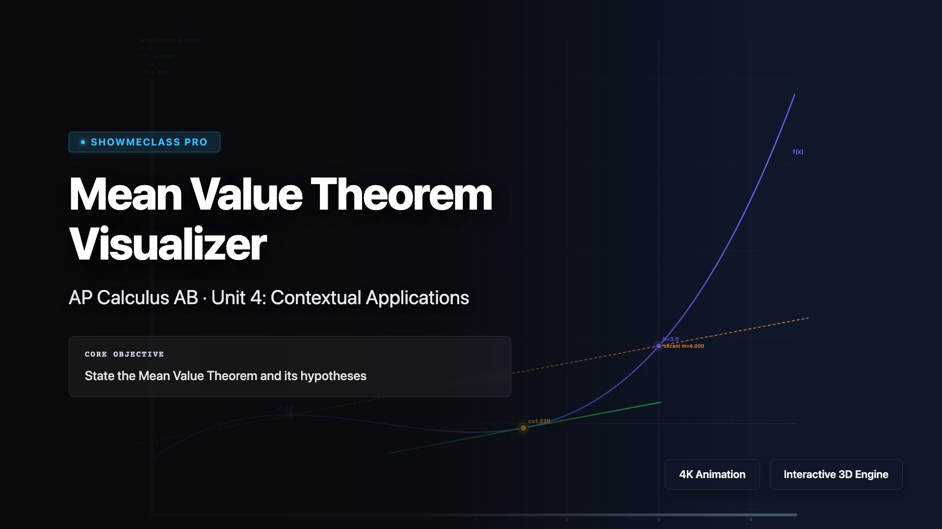
Mean Value Theorem Visualizer
Visualize the Mean Value Theorem (MVT), which guarantees that for a continuous and differentiable function on [a,b], there exists at least one point c where f'(c) = (f(b)-f(a))/(b-a). Explore how the instantaneous rate of change equals the average rate of change at some interior point. Understand MVT's applications in proving inequalities, analyzing motion, and establishing fundamental results like the constant difference theorem.
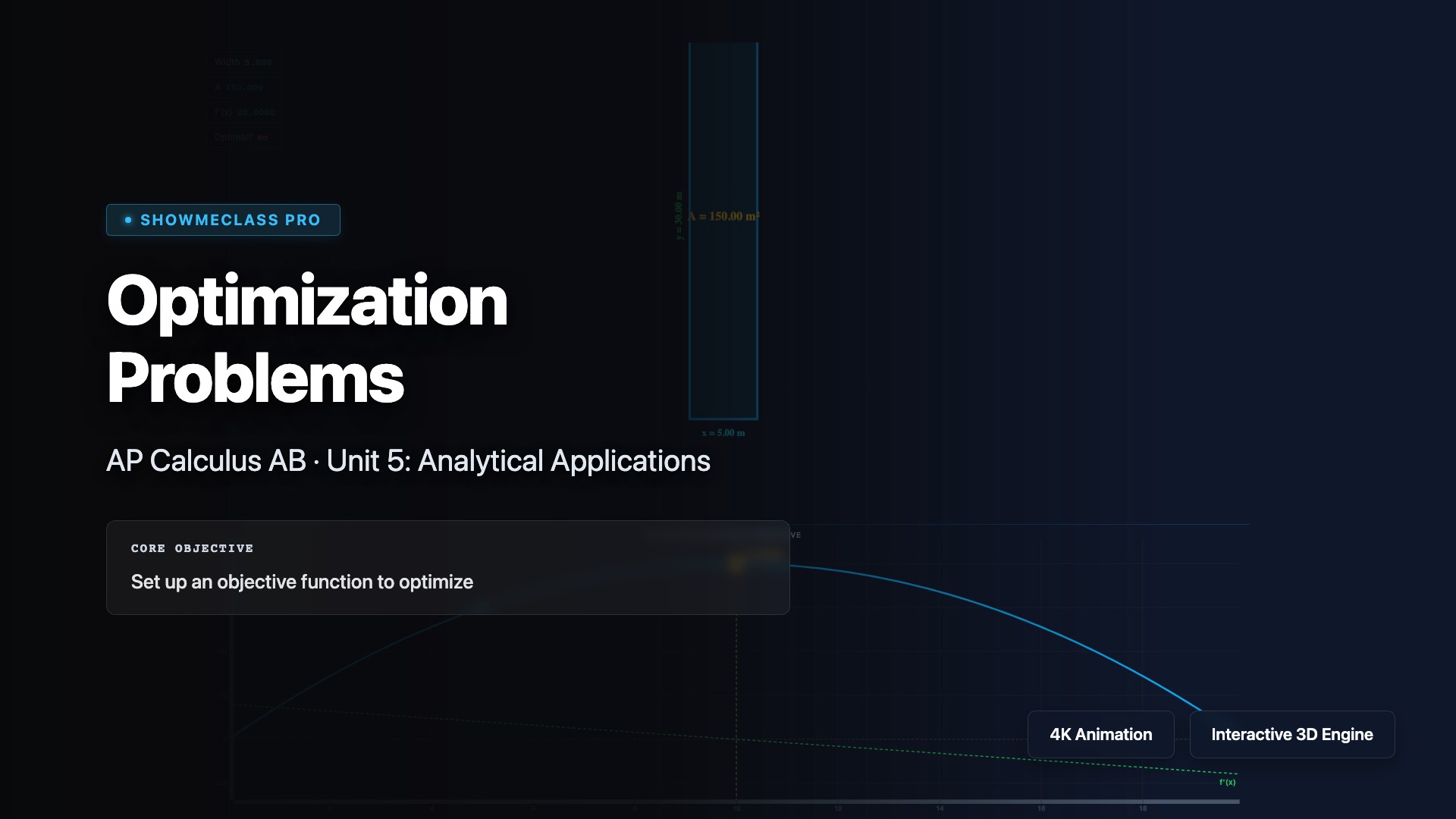
Optimization Problems
Solve optimization problems by finding absolute and relative extrema using calculus techniques. Learn to identify constraints, write objective functions, take derivatives, find critical points using f'(x) = 0, and apply the first or second derivative test. Explore real-world applications including maximizing area, minimizing cost, optimizing volume, and finding shortest distances in geometry, physics, and economics.
Related Rates Visualizer
Solve related rates problems where multiple quantities change with respect to time and are connected by an equation. Use implicit differentiation with respect to time to find how one rate of change relates to another. Visualize classic scenarios like ladder sliding down walls, water filling conical tanks, expanding circles, and moving shadows, applying the chain rule to connect dy/dt, dx/dt, and geometric relationships.
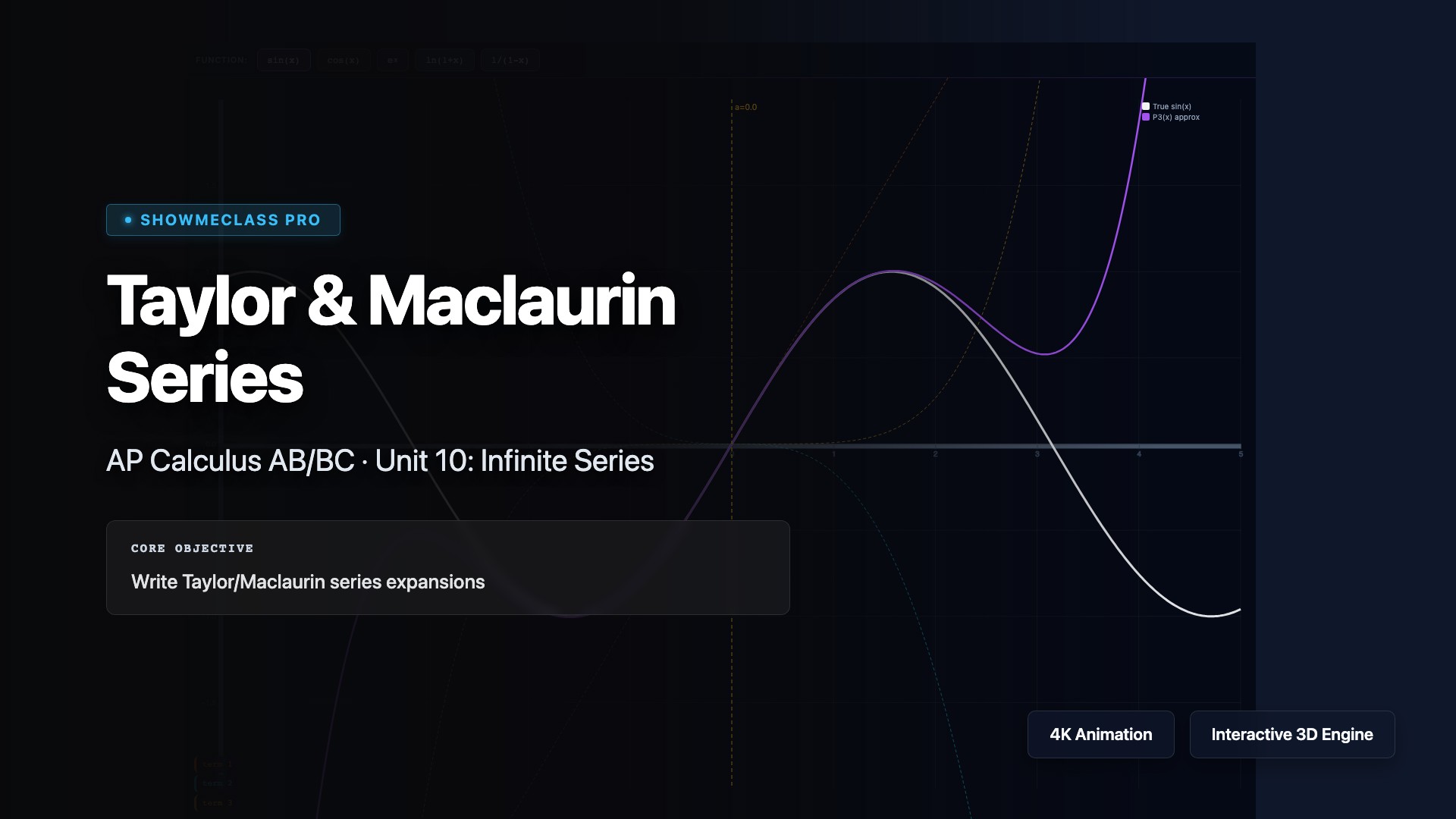
Taylor Series
Explore Taylor and Maclaurin series, which approximate functions as infinite polynomials using derivatives at a single point. Visualize how f(x) ≈ f(a) + f'(a)(x-a) + f''(a)(x-a)²/2! + ... converges to the original function. Understand how adding more terms improves accuracy, and learn common series for e^x, sin(x), cos(x), and ln(1+x). Practice finding intervals of convergence and estimating error bounds.
Volumes w/ Known Cross Sections
Calculate volumes of solids with known cross-sectional shapes perpendicular to an axis using integration. Visualize how V = ∫[a to b] A(x)dx sums infinitely many cross-sectional areas—squares, rectangles, semicircles, equilateral triangles, and isosceles right triangles. Understand how the base region determines the limits of integration and how the cross-section shape determines the area function A(x).
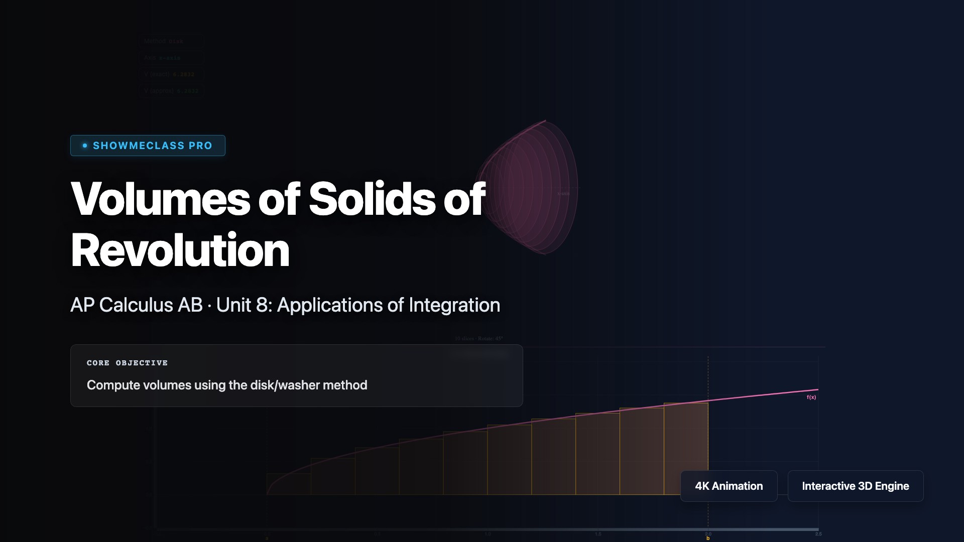
Volumes of Solids of Revolution
Calculate volumes of three-dimensional solids formed by rotating regions around axes using disk, washer, and shell methods. Visualize the disk method V = π∫[a to b] [R(x)]²dx for solids without holes, the washer method V = π∫[a to b] ([R(x)]² - [r(x)]²)dx for solids with holes, and the shell method V = 2π∫[a to b] x·h(x)dx for rotation around vertical axes. Master choosing the most efficient method for each problem.
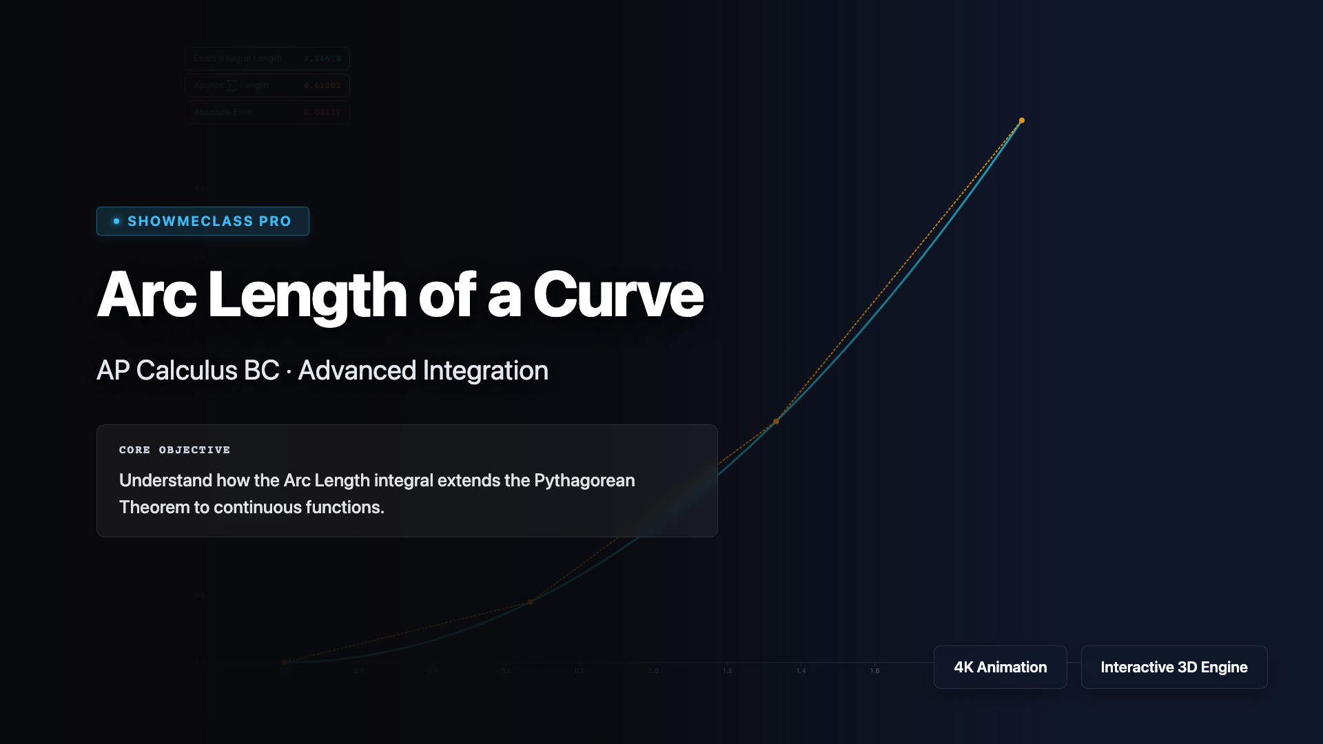
Arc Length of a Curve
Calculate the arc length of curves using integration and the distance formula. Derive and apply the arc length formula L = ∫[a to b] √(1 + [f'(x)]²)dx for functions y = f(x), or L = ∫[α to β] √([dx/dt]² + [dy/dt]²)dt for parametric curves. Understand how the Pythagorean theorem leads to this formula by summing infinitesimal line segments along the curve.
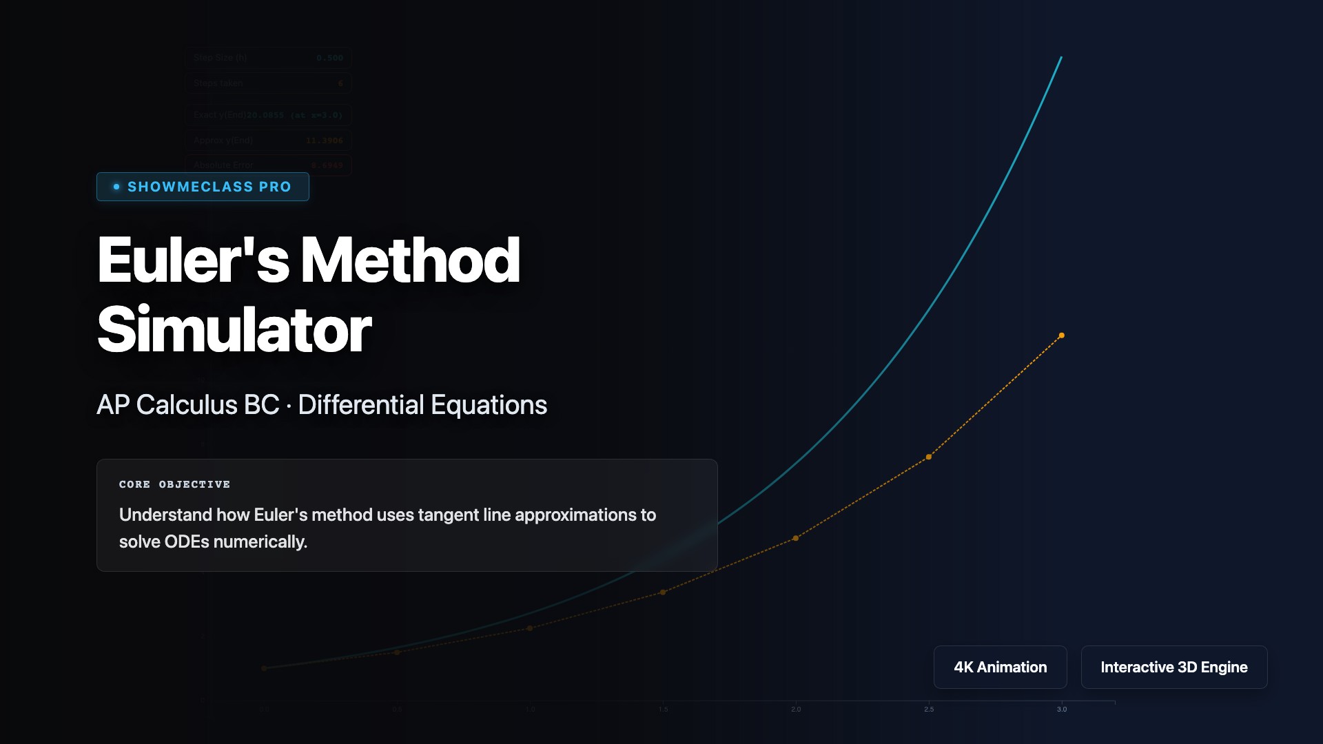
Euler's Method Simulator
Approximate solutions to differential equations using Euler's method, a numerical technique that uses tangent line approximations. Starting from an initial condition, iteratively calculate y_{n+1} = y_n + f(x_n, y_n)·Δx to trace the solution curve. Visualize how smaller step sizes improve accuracy, understand accumulation of error, and explore applications where analytical solutions are difficult or impossible to find.
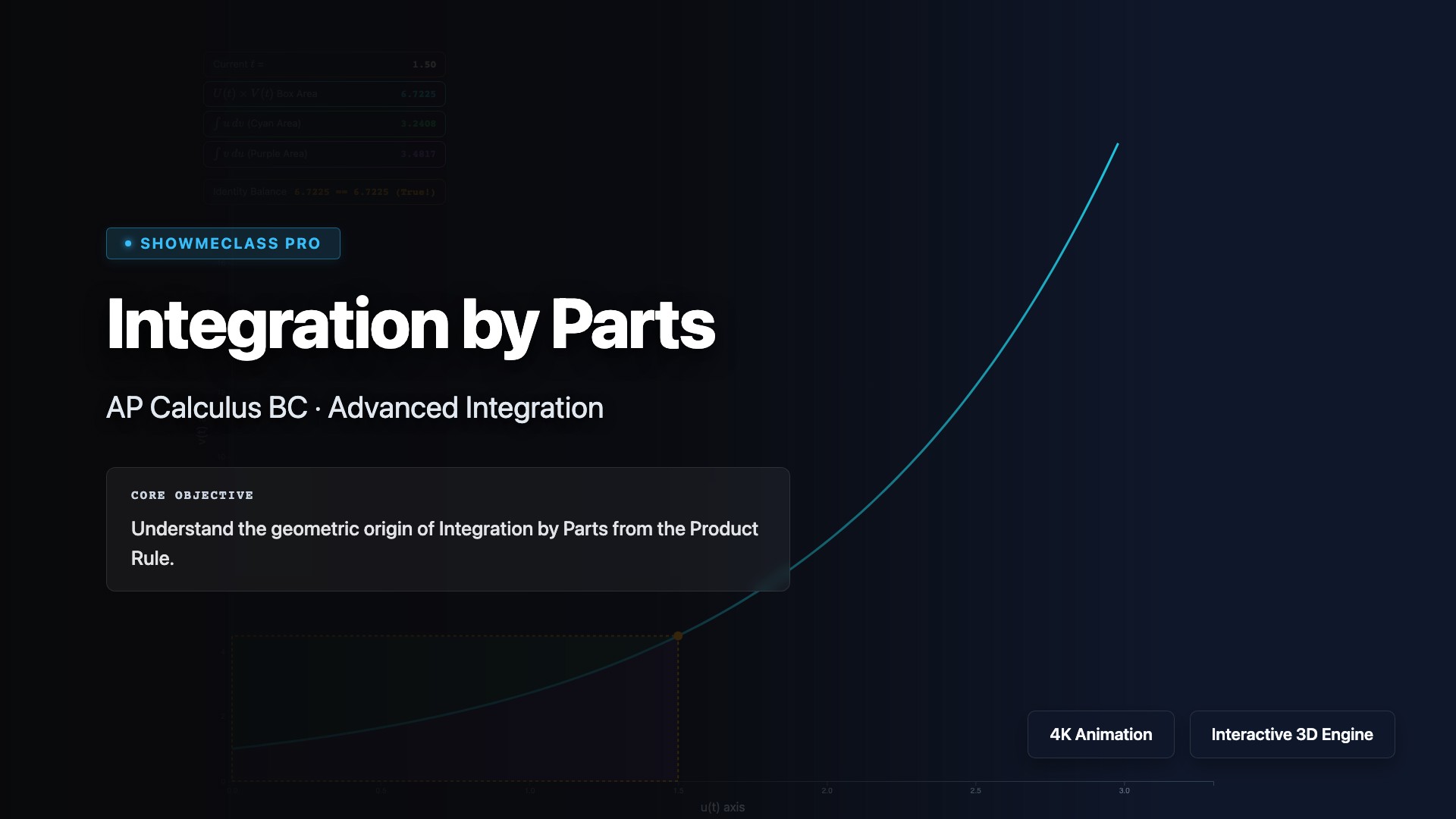
Integration by Parts
Master integration by parts, derived from the product rule for differentiation, using the formula ∫u dv = uv - ∫v du. Learn strategic selection of u and dv using the LIATE priority (Logarithmic, Inverse trig, Algebraic, Trigonometric, Exponential). Practice solving integrals involving products of functions, handling repeated applications, and recognizing when tabular integration or reduction formulas provide efficient solutions.
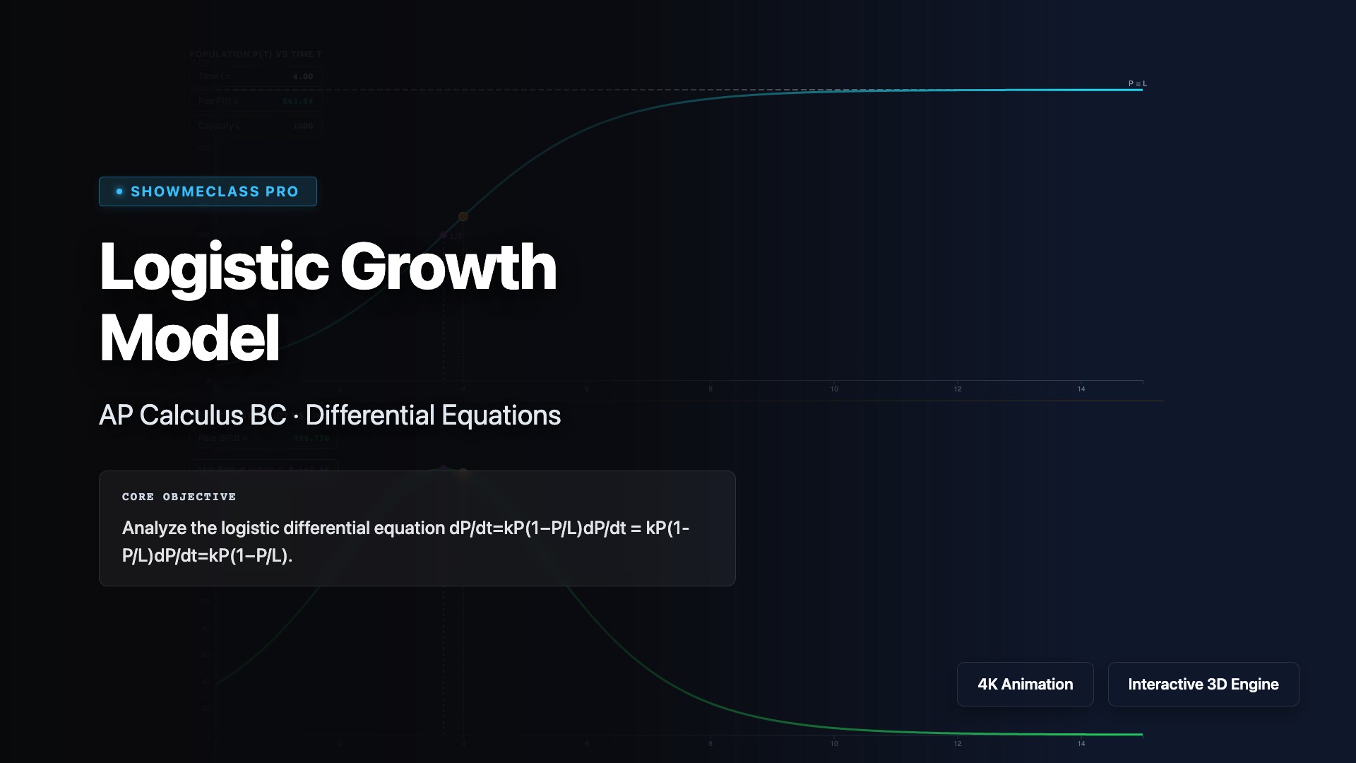
Logistic Growth Model
Model population growth with limited resources using the logistic differential equation dP/dt = kP(1 - P/M), where M is the carrying capacity. Visualize the S-shaped logistic curve P(t) = M/(1 + Ae^(-kt)) and understand how growth rate is fastest at P = M/2. Explore applications in ecology, epidemiology, and economics where growth is constrained by environmental factors, resource availability, or market saturation.
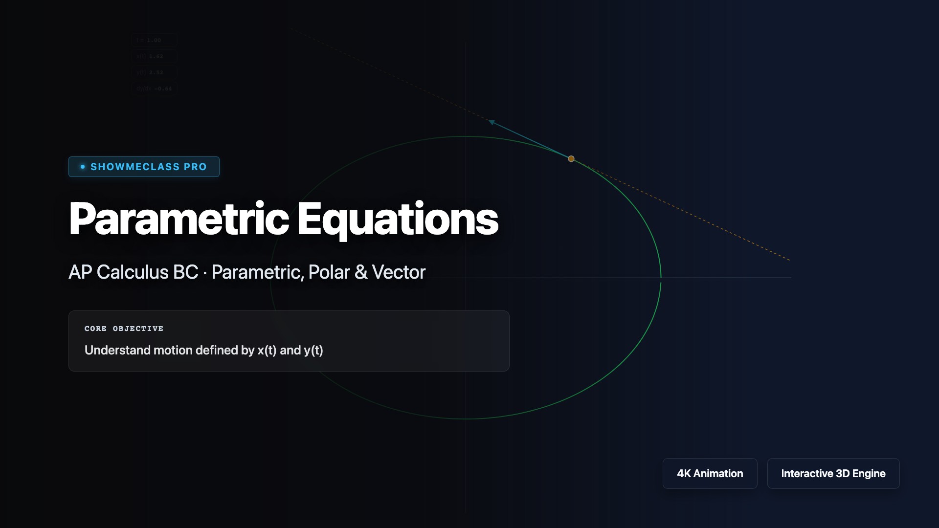
Parametric Equations
Explore parametric equations where x and y are both functions of a parameter t, enabling representation of curves that fail the vertical line test. Calculate derivatives dy/dx = (dy/dt)/(dx/dt) and second derivatives for analyzing concavity. Find arc length, speed, and velocity vectors. Visualize classic parametric curves like cycloids, ellipses, and Lissajous figures, and understand applications in physics for modeling projectile motion and planetary orbits.