Polar Tangent Lines & Slope
Visualize dy/dx for polar curves r=f(θ) using the chain rule conversion to Cartesian. Shows tangent lines, radial vectors, and identifies horizontal/vertical tangents on Cardioid, Rose, Limaçon, and Lemniscate curves.
Visualize dy/dx for polar curves r=f(θ) using the chain rule conversion to Cartesian. Shows tangent lines, radial vectors, and identifies horizontal/vertical tangents on Cardioid, Rose, Limaçon, and Lemniscate curves.

Estimate the error when approximating infinite series with partial sums using error bound theorems. For alternating series, the error is bounded by the absolute value of the first omitted term. For Taylor series, use the Lagrange error bound |Rₙ(x)| ≤ M|x-a|^(n+1)/(n+1)! where M is the maximum of |f^(n+1)| on the interval. Practice determining how many terms are needed to achieve a desired accuracy.

Analyze motion in two dimensions using vector-valued functions for position r(t) = ⟨x(t), y(t)⟩. Calculate velocity vectors v(t) = r'(t), acceleration vectors a(t) = v'(t), and speed |v(t)| = √[(dx/dt)² + (dy/dt)²]. Visualize how velocity is tangent to the path, acceleration points toward concavity, and understand applications in projectile motion, planetary orbits, and particle kinematics.

Calculate the arc length of curves using integration and the distance formula. Derive and apply the arc length formula L = ∫[a to b] √(1 + [f'(x)]²)dx for functions y = f(x), or L = ∫[α to β] √([dx/dt]² + [dy/dt]²)dt for parametric curves. Understand how the Pythagorean theorem leads to this formula by summing infinitesimal line segments along the curve.
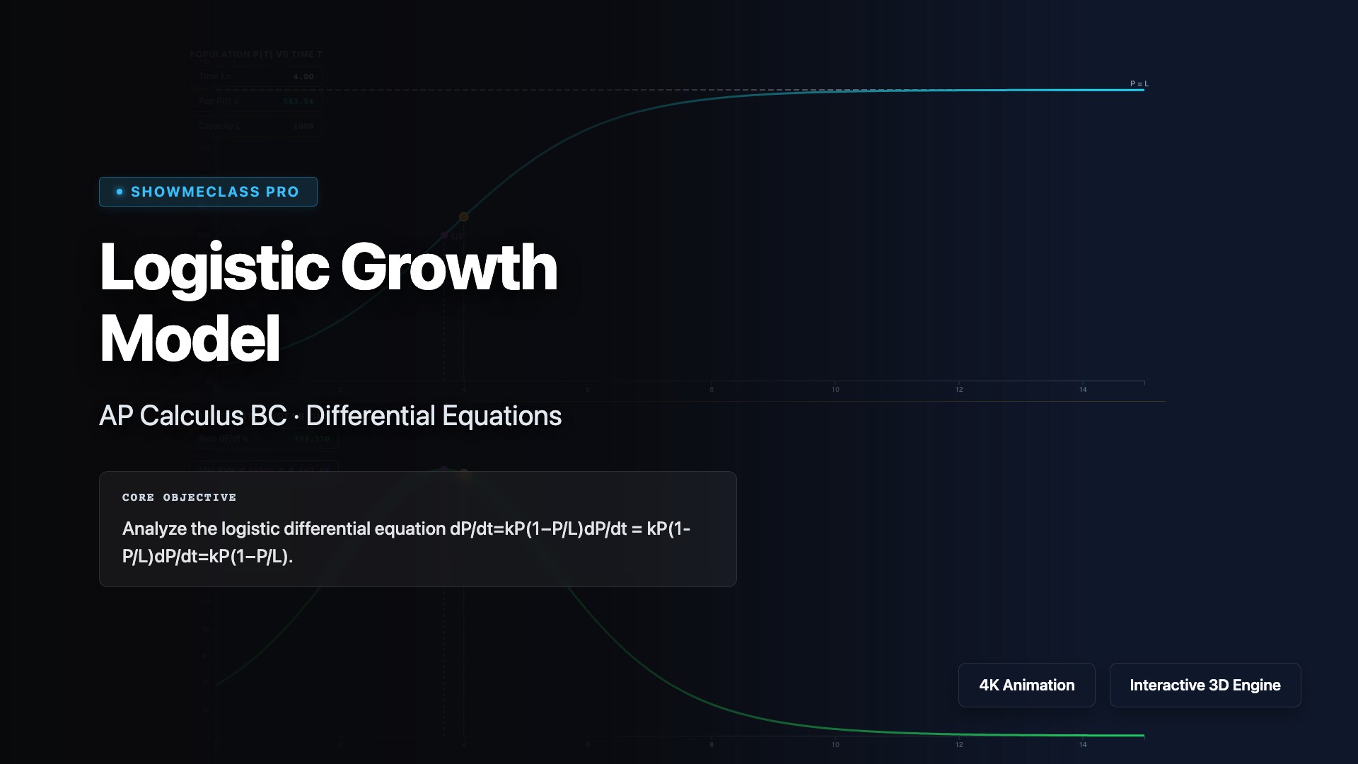
Model population growth with limited resources using the logistic differential equation dP/dt = kP(1 - P/M), where M is the carrying capacity. Visualize the S-shaped logistic curve P(t) = M/(1 + Ae^(-kt)) and understand how growth rate is fastest at P = M/2. Explore applications in ecology, epidemiology, and economics where growth is constrained by environmental factors, resource availability, or market saturation.