
Showing 12 results

Polar Area & Curves
Graph and analyze curves in polar coordinates where r = f(θ), and calculate areas using A = (1/2)∫[α to β] [r(θ)]²dθ. Visualize classic polar curves including circles, cardioids, limaçons, rose curves, and lemniscates. Understand symmetry tests, find tangent lines using dr/dθ, and explore how polar coordinates naturally describe curves with rotational symmetry that are complex in Cartesian form.

Series Convergence Tests
Master the convergence tests for infinite series including the nth-term test, geometric series test, p-series test, integral test, comparison tests, limit comparison test, alternating series test, ratio test, and root test. Learn when to apply each test, understand their conditions and conclusions, and develop strategies for determining whether ∑aₙ converges or diverges. Practice identifying series types and selecting the most efficient test.

Infinite Series Error Bounds
Estimate the error when approximating infinite series with partial sums using error bound theorems. For alternating series, the error is bounded by the absolute value of the first omitted term. For Taylor series, use the Lagrange error bound |Rₙ(x)| ≤ M|x-a|^(n+1)/(n+1)! where M is the maximum of |f^(n+1)| on the interval. Practice determining how many terms are needed to achieve a desired accuracy.
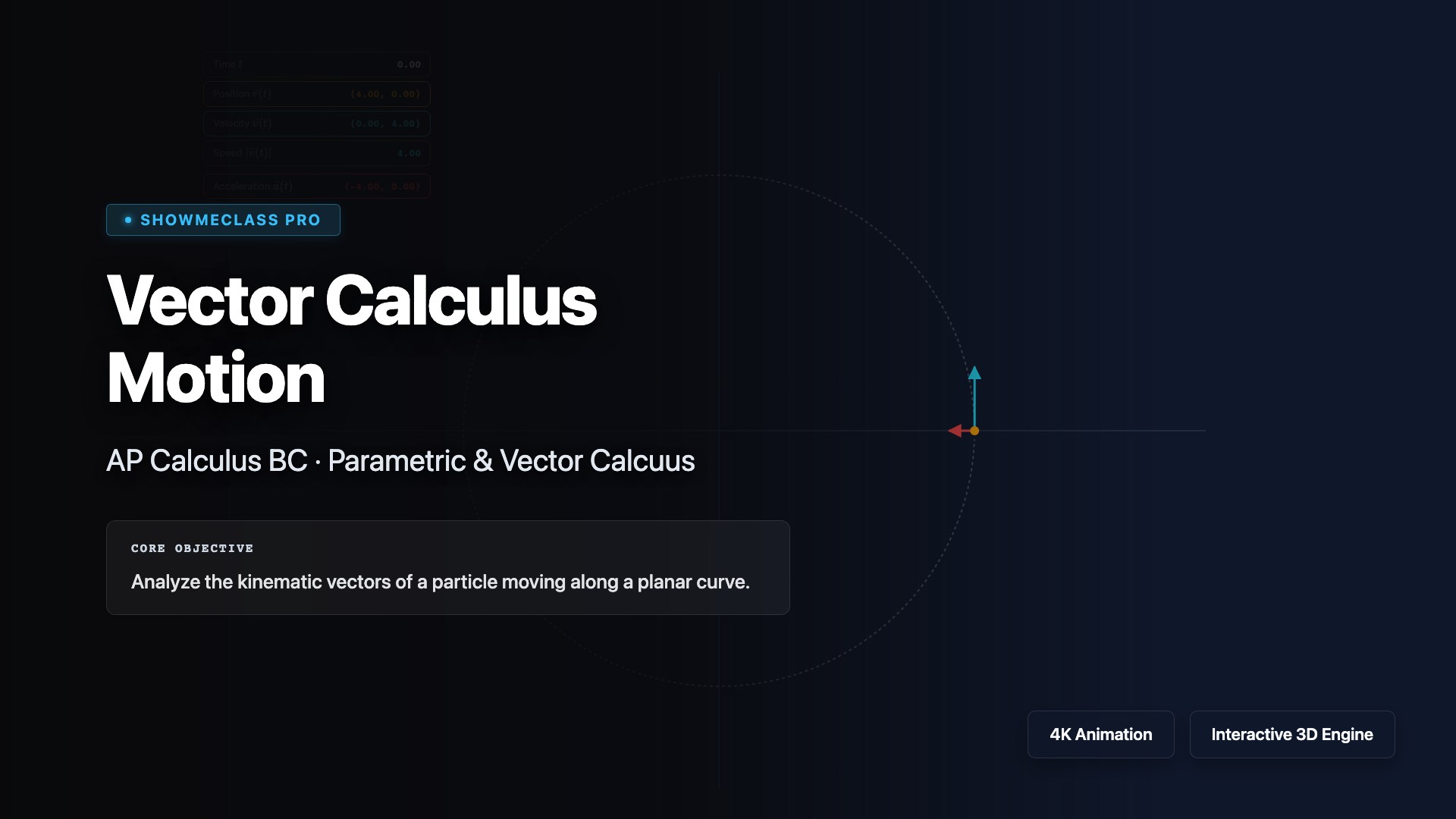
Vector Calculus Motion
Analyze motion in two dimensions using vector-valued functions for position r(t) = ⟨x(t), y(t)⟩. Calculate velocity vectors v(t) = r'(t), acceleration vectors a(t) = v'(t), and speed |v(t)| = √[(dx/dt)² + (dy/dt)²]. Visualize how velocity is tangent to the path, acceleration points toward concavity, and understand applications in projectile motion, planetary orbits, and particle kinematics.
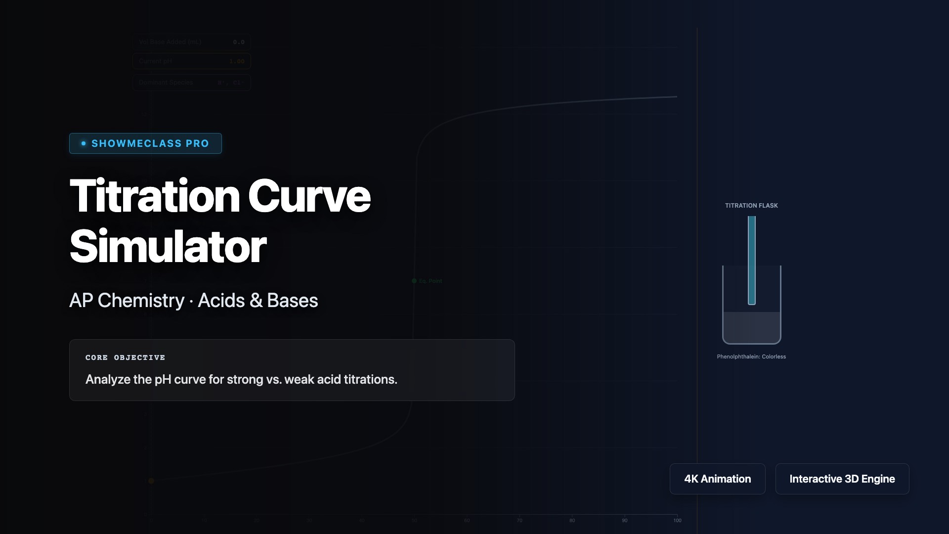
Titration Curve Simulator
Simulate acid-base titrations and analyze pH curves for strong-strong, weak-strong, and polyprotic titrations. Visualize how pH changes as titrant is added, identify equivalence points, buffer regions, and half-equivalence points where pH = pKa. Understand the Henderson-Hasselbalch equation, calculate buffer capacity, and select appropriate indicators based on their pKa values and the pH at equivalence.

Atomic Orbital Shapes
Visualize the three-dimensional shapes of atomic orbitals (s, p, d, and f) that describe the probability distribution of electrons around the nucleus. Explore how quantum numbers (n, l, mₗ, mₛ) define orbital characteristics including energy level, shape, orientation, and electron spin. Understand the relationship between orbital shapes and chemical bonding, electron configuration, and the periodic table structure.
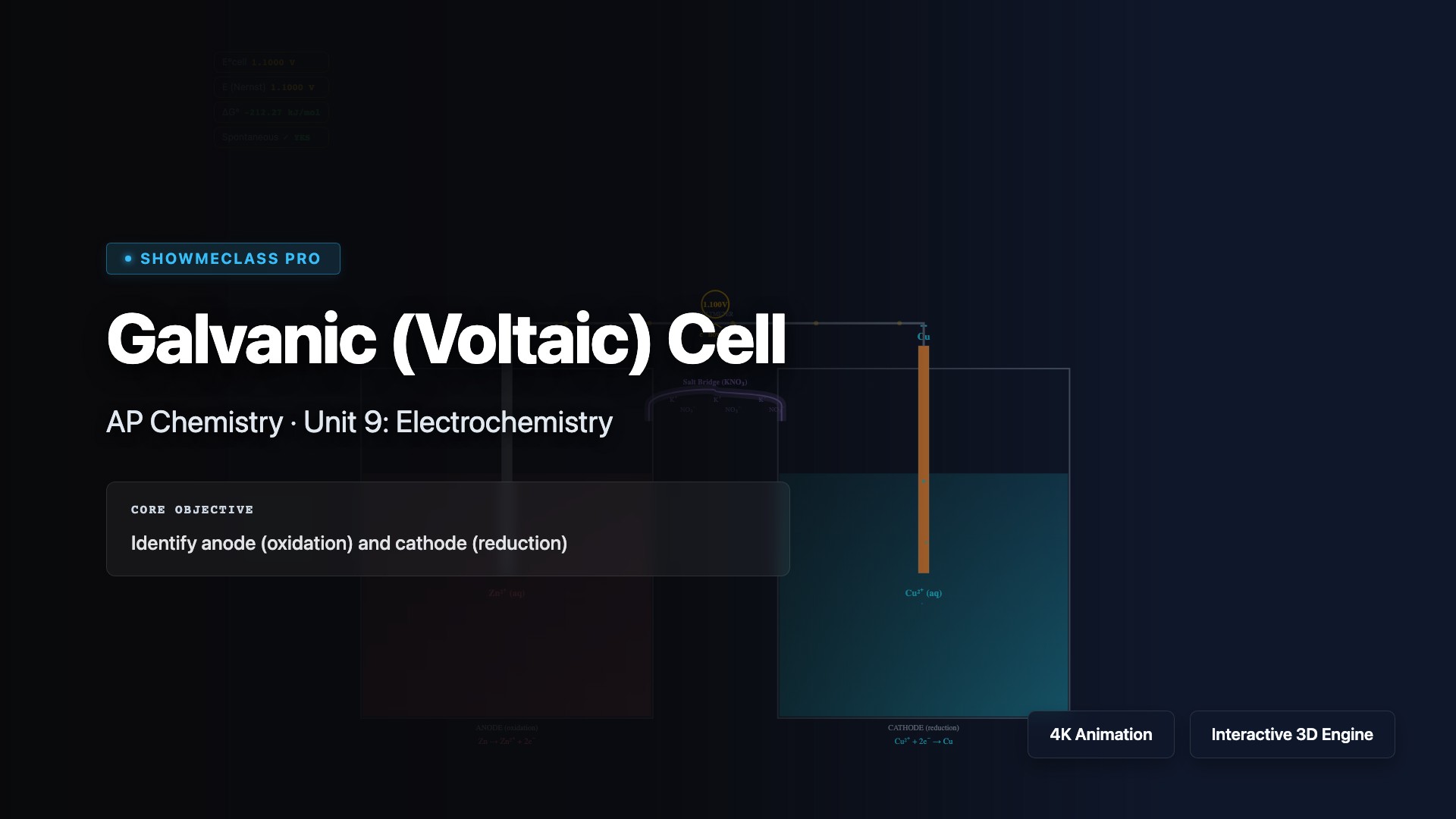
Galvanic (Voltaic) Cell
Explore galvanic (voltaic) cells that convert chemical energy into electrical energy through spontaneous redox reactions. Visualize electron flow from anode (oxidation) to cathode (reduction), ion movement through the salt bridge, and calculate cell potential using E°cell = E°cathode - E°anode. Understand the Nernst equation, concentration effects on voltage, and applications in batteries and fuel cells.

Electron Configuration
Build electron configurations for atoms and ions using the Aufbau principle, Hund's rule, and the Pauli exclusion principle. Visualize how electrons fill orbitals in order of increasing energy (1s, 2s, 2p, 3s, 3p, 4s, 3d...), understand noble gas notation shortcuts, and identify valence electrons. Explore exceptions like chromium and copper, and connect electron configuration to periodic trends and chemical reactivity.

Enthalpy vs Entropy (ΔG)
Explore the relationship between enthalpy (ΔH), entropy (ΔS), and Gibbs free energy (ΔG) using the equation ΔG = ΔH - TΔS. Understand how temperature affects spontaneity: exothermic reactions with increasing entropy are always spontaneous, while endothermic reactions with decreasing entropy are never spontaneous. Visualize how ΔG < 0 indicates spontaneous processes, ΔG = 0 represents equilibrium, and ΔG > 0 means non-spontaneous reactions.
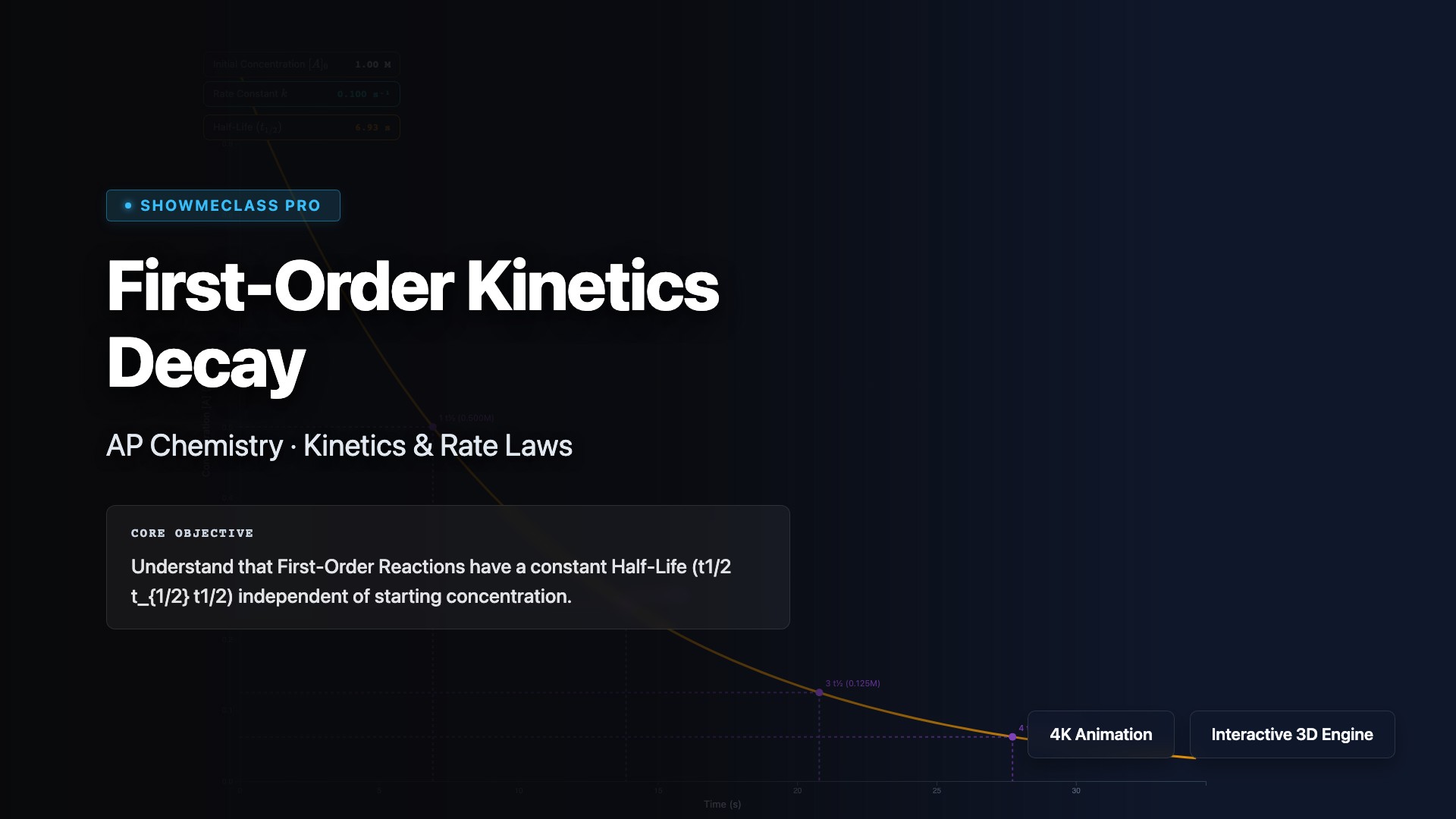
First-Order Kinetics Decay
Analyze first-order reactions where the rate depends linearly on one reactant concentration: rate = k[A]. Visualize exponential decay using the integrated rate law ln[A]t = ln[A]₀ - kt, and understand that first-order reactions have constant half-life t₁/₂ = 0.693/k independent of initial concentration. Explore applications in radioactive decay, drug metabolism, and chemical decomposition reactions.
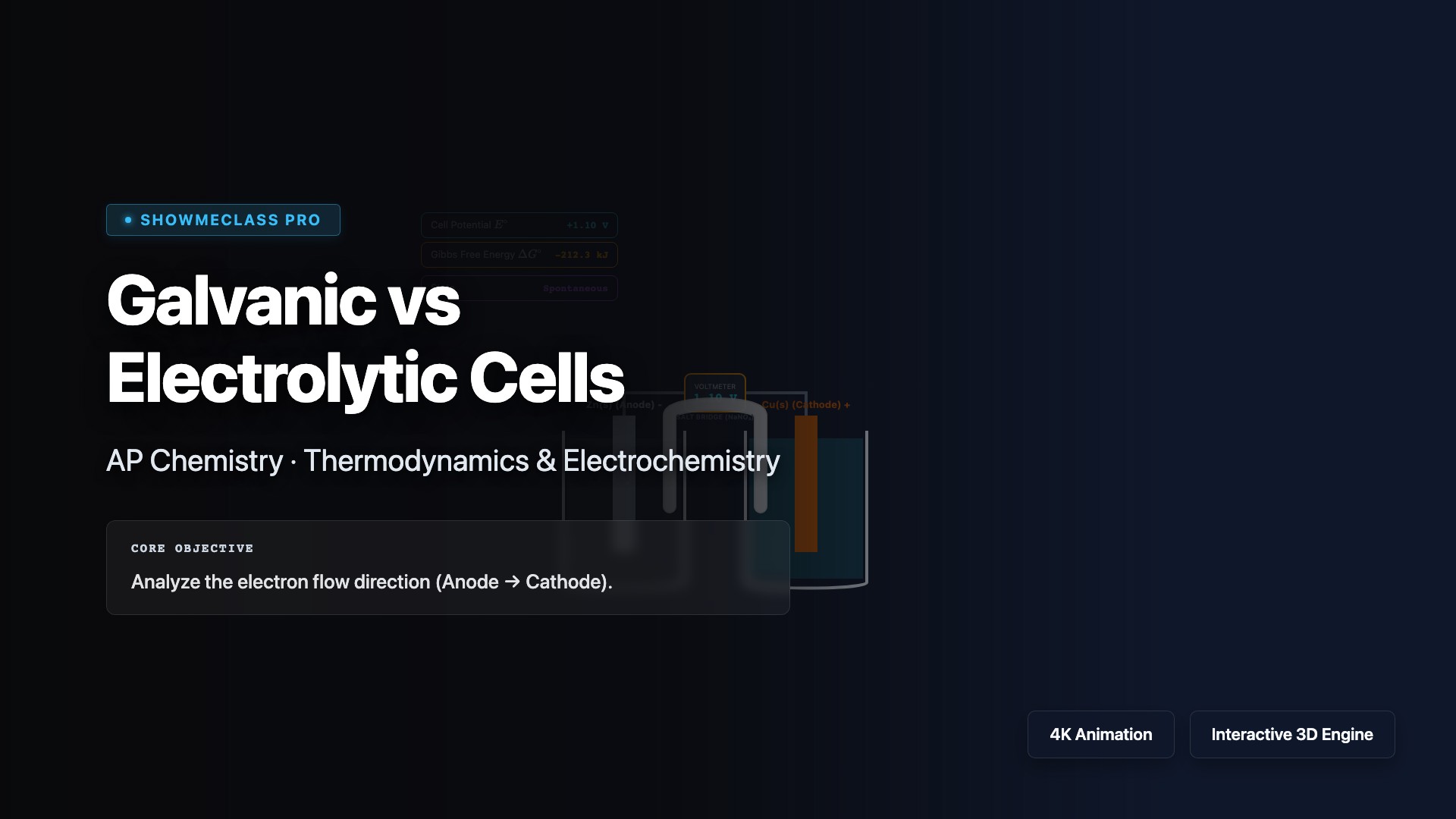
Galvanic vs Electrolytic Cells
Compare galvanic cells (spontaneous, ΔG < 0, generate electricity) with electrolytic cells (non-spontaneous, ΔG > 0, require external voltage). Visualize how galvanic cells convert chemical energy to electrical energy in batteries, while electrolytic cells use electrical energy to drive non-spontaneous reactions in electroplating, electrolysis, and metal purification. Understand electrode polarity differences and the role of external power sources.
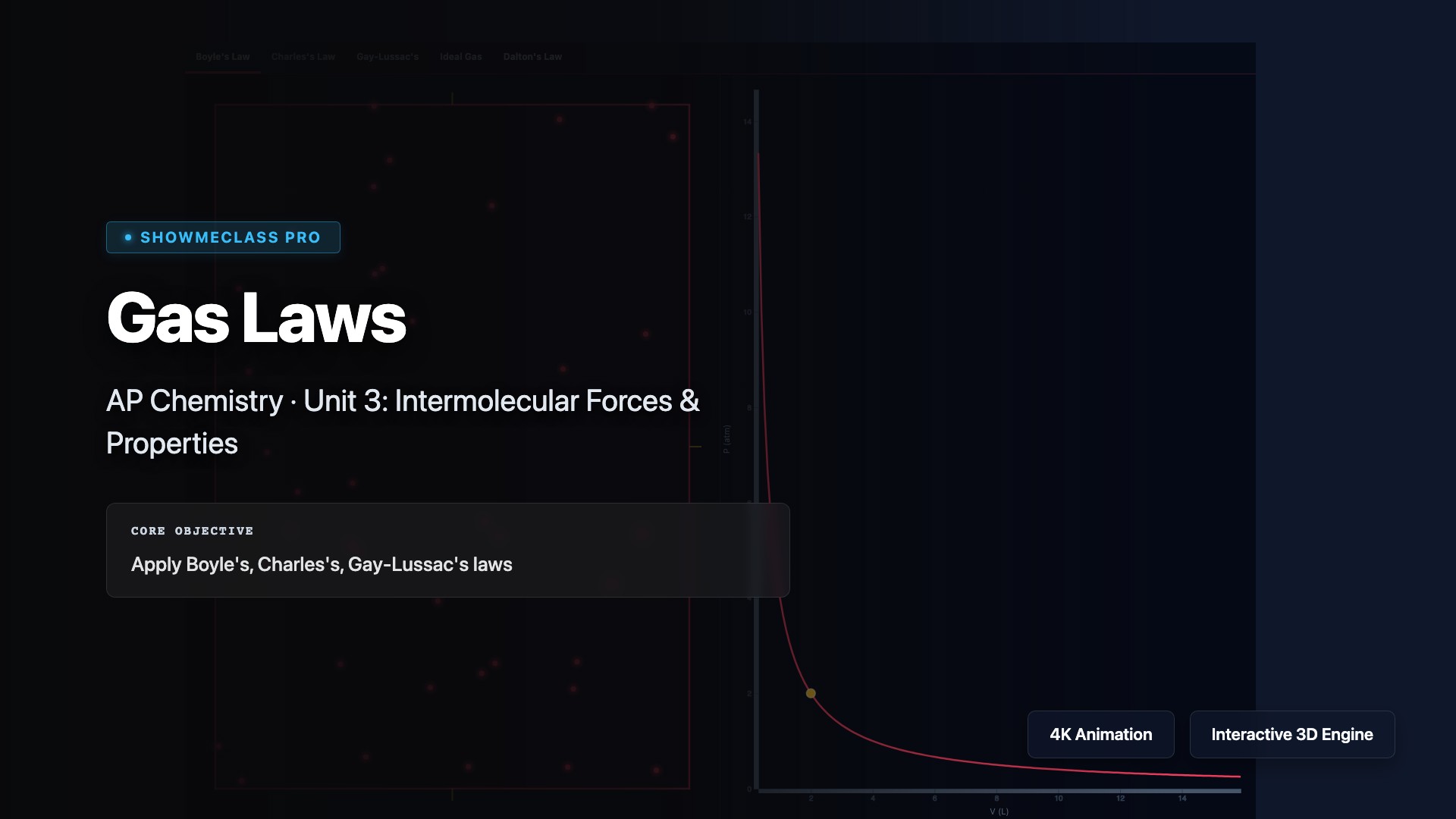
Gas Laws
Explore the fundamental gas laws that describe relationships between pressure, volume, temperature, and amount of gas. Visualize Boyle's Law (P₁V₁ = P₂V₂), Charles's Law (V₁/T₁ = V₂/T₂), Gay-Lussac's Law (P₁/T₁ = P₂/T₂), Avogadro's Law (V₁/n₁ = V₂/n₂), and the Combined Gas Law. Understand how these individual laws combine to form the Ideal Gas Law PV = nRT.